In response to the rapidly evolving financial market and the escalating concern surrounding credit risk in digital financial institutions, this project addresses the urgency for accurate credit risk prediction models. Traditional methods such as Neural network models, kernel-based virtual machines, Z-score, and Logit (logistic regression model) have all been used, but their results have proven less than satisfactory. The project focuses on developing a credit scoring model specifically tailored for digital financial institutions, by leveraging a hybrid model that combines long short-term memory (LSTM) networks with recurrent neural networks (RNN). This innovative approach capitalizes on the strengths of the Long-Short Term Memory (LSTM) for long-term predictions and Recurrent Neural Network (RNN) for its recurrent neural network capabilities. A key component of the approach is feature selection, which entails extracting a subset of pertinent features from the credit risk data using RNN in order to help classify loan applications. The researcher chose to use data from Kaggle to study and compare the efficacy of different models. The findings reveal that the RNN-LSTM hybrid model outperforms other RNNs, LSTMs, and traditional models. Specifically, the hybrid model demonstrated distinct advantages, showcasing higher accuracy and a superior Area Under the Curve (AUC) compared to individual RNN and LSTM models. While RNN and LSTM models exhibited slightly lower accuracy individually, their combination in the hybrid model proved to be the optimal choice. In summary, the RNN-LSTM hybrid model developed stands out as the most effective solution for predicting credit risk in digital financial institutions, surpassing the performance of standalone RNN and LSTM models as well as traditional methodologies. This research contributes valuable insights for banks, regulators, and investors seeking robust credit risk assessment tools in the dynamic landscape of digital finance.
| Published in | International Journal of Statistical Distributions and Applications (Volume 10, Issue 2) |
| DOI | 10.11648/j.ijsd.20241002.11 |
| Page(s) | 16-24 |
| Creative Commons |
This is an Open Access article, distributed under the terms of the Creative Commons Attribution 4.0 International License (http://creativecommons.org/licenses/by/4.0/), which permits unrestricted use, distribution and reproduction in any medium or format, provided the original work is properly cited. |
| Copyright |
Copyright © The Author(s), 2024. Published by Science Publishing Group |
Neural Network (NN), Machine Learning (ML), Deep Learning (DL), Area Under the Curve (AUC), Recurrent Neural Network (RNN), Convolutional Neural Network (CNN), Long-Short Term Memory (LSTM)
3.1. Recurrent Neural Network (RNN)
3.2. Feature Selection Using Recurrent Neural Networks (RNN)
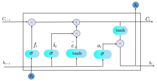
3.3. Long Short-Term Memory (LSTM) Model
3.4. The Working Model (RNN-LSTM Hybrid Model)
3.5. Evaluation Measures
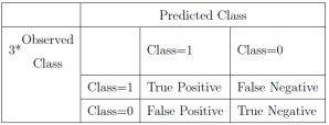
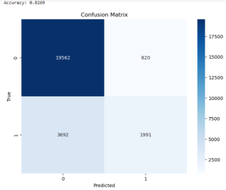
3.5.1. Confusion Matrix
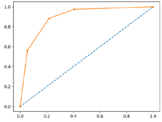
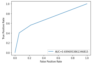
3.5.2. Receiver Operating Characteristic (ROC) Curve
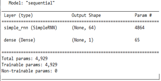
4.1. Recurrent Neural Network Results
Features | GINI Index |
|---|---|
Loan intent | 1.9519195556640625 |
Person age | 1.7832162380218506 |
Person income | 1.752898097038269 |
Loan amount | 1.6746004819869995 |
Loan percent income | 1.668798804283142 |
Loan grade | 1.6389334201812744 |
Person home ownership | 1.53562784194963 |
Loan interest rate | 1.501058578491211 |
Person employment length | 1.424591064453125 |
Cb person credit history length | 1.2153666019439697 |
4.2. Long Short-Term Memory (LSTM) Model Results
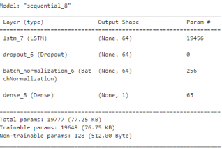
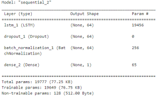
4.3. RNN-LSTM Hybrid Model Results
4.4. Evaluation of the Models' Performance
MODEL | SENSITIVITY | SPECIFICITY | F1-SCORE | ACCURACY (%) |
|---|---|---|---|---|
RNN | 0.8060 | 0.9560 | 0.1469 | 78.35 |
LSTM | 0.8607 | 0.9601 | 0.5088 | 81.07 |
RNN-LSTM HYBRID | 0.8909 | 0.9670 | 0.6059 | 82.69 |
MODEL | AREA UNDER THE ROC CURVE (AUC) |
|---|---|
RNN | 0.6166 |
LSTM | 0.6485 |
RNN-LSTM HYBRID | 0.6997 |
| [1] | Addo, P., Guegan, D. & Hassani, B. (2018). Credit risk analysis using machine and deep learning models. Risks, 6(2), |
| [2] | Akkok, S. (2012). An empirical comparison of conventional techniques, neural networks and the three stage hybrid adaptive neuro fuzzyinference system (anfis) model for credit scoring analysis: The case of Turkish credit card data. European Journal of Operational Research, 222(1), 168-178 |
| [3] | Alborzi, M & Khanbabaei, M. (2016). Using data mining and neural networks techniques to propose a new hybrid customer behaviour analysis and credit scoring model in banking services based on a developed rfm analysis method. Internstional Journal of Business Information Systems, 23(1), 1-22. |
| [4] | Altman, E. (1968). Financial ratios, discriminant analysis and the prediction of corporate bankruptcy. The journal of Finance, 23(4), 589-609. |
| [5] | Angelini, E., DiTollo, G. & Roli, A. (2008). A neural network approach for credit ris evaluation. The quarterly review of economics and finance, 48(4), 733-755. |
| [6] | Asgari, E.,, Bastani, K. & Namavari, H.,. (2019). Wide and deep learning for peer and peer lending. Expert Systems with Applications, 134, 209-224. |
| [7] | Basuvarai, M., & Jegadeeshwaran, M. (2020). Effect of internal factors of credit risk on perfomance indicators of Indian public sectors banks after global financial recession. Journal of the Social Sciences 48(3). |
| [8] | Breiman, L. & Ihaka, R. (1984). Nonlinear discriminant analysis via scaling and ace. Department of statistics, University of California Davis One Shields. |
| [9] | Brummelhuis, R., & Luo, Z. (2017). Cds rate construction methods by machine learning techniques. arXiv preprint 1705.0689954. |
| [10] |
Butaru, F., Chen, Q., Clark, B., Das, S., Lo, A. W. & Siddique, A. (2016). Risk and risk management in the credit card industry. Journal of Banking and Finance. 72, 218-239.
https://www.nber.org/system/files/working_papers/w21305/w21305.pdf |
| [11] | Chauhan, N., Ravi, V., & Chandra, D. K. (2009). Differential evolution trained wavelet neural networks: Application to bankruptcy prediction in banks.. Expert systems with Applications, 36(4), 7659-7665. |
| [12] | Cui, Y. & Liu, L. (2022). Investor Sentiment-aware prediction model for p2p lending indicators based on lstm. Plos one, 17(1), e0262539. |
| [13] | Dietterich, T. G., & Kong, E. B. (1995). Machine learning bias, statistical bias and statistical variance of decision tree algorithms. Tech Rep. Citeseer. |
| [14] | Fausett, L. V. (1984). An analysis of mathematical models of underground coal gasification. University of Wyoming. |
| [15] | Fernandez-Delgado, M. C. (2014). Do we need hundreds of classifiers to solve problems? The journal of Machine learning research, 15(1), 3133-3181. |
| [16] | Fogarty, D. J. (2012). Using genetic algorithms for credit scoring system maintenance functions. International Journal of Artificial Intelligence & Applications 3(6), 1. |
| [17] | Guo, Y., Mei, J., Pan, Z., Liu, H., & Li, W. (2022). Adaptively promoting diversity in a novel ensemble method for imbalanced credit-risk evaluation.. Mathematics, 10(11), 1790. |
| [18] | Gupta, D. K., & Goyal, S. (2018). Credit risk prediction using artificial neural network algorithm. International Journal of modern Education and Computer Science, 10(5), 9. |
| [19] | Hidasi, B., Karatzoglou, A., Baltrunas, L., & Tikk, D. (2015). Session-based recommendations with recurrent neural networks. arXiv preprint ArXiv:, 1511.06939. |
| [20] | Hsieh, N. C., & Hung, L. P. (2010). A data driven ensemble classifier for credit scoring analysis. Expert systems with applications, 37(1), 534-545. |
APA Style
Musyoka, G. K., Waititu, A. G., Imboga, H. (2024). Credit Risk Modelling Using RNN-LSTM Hybrid Model for Digital Financial Institutions . International Journal of Statistical Distributions and Applications, 10(2), 16-24. https://doi.org/10.11648/j.ijsd.20241002.11
ACS Style
Musyoka, G. K.; Waititu, A. G.; Imboga, H. Credit Risk Modelling Using RNN-LSTM Hybrid Model for Digital Financial Institutions . Int. J. Stat. Distrib. Appl. 2024, 10(2), 16-24. doi: 10.11648/j.ijsd.20241002.11
AMA Style
Musyoka GK, Waititu AG, Imboga H. Credit Risk Modelling Using RNN-LSTM Hybrid Model for Digital Financial Institutions . Int J Stat Distrib Appl. 2024;10(2):16-24. doi: 10.11648/j.ijsd.20241002.11
@article{10.11648/j.ijsd.20241002.11,
  author = {Gabriel King’auwi Musyoka and Antony Gichuhi Waititu and Herbert Imboga},
  title = {Credit Risk Modelling Using RNN-LSTM Hybrid Model for Digital Financial Institutions
},
  journal = {International Journal of Statistical Distributions and Applications},
  volume = {10},
  number = {2},
  pages = {16-24},
  doi = {10.11648/j.ijsd.20241002.11},
  url = {https://doi.org/10.11648/j.ijsd.20241002.11},
  eprint = {https://article.sciencepublishinggroup.com/pdf/10.11648.j.ijsd.20241002.11},
  abstract = {In response to the rapidly evolving financial market and the escalating concern surrounding credit risk in digital financial institutions, this project addresses the urgency for accurate credit risk prediction models. Traditional methods such as Neural network models, kernel-based virtual machines, Z-score, and Logit (logistic regression model) have all been used, but their results have proven less than satisfactory. The project focuses on developing a credit scoring model specifically tailored for digital financial institutions, by leveraging a hybrid model that combines long short-term memory (LSTM) networks with recurrent neural networks (RNN). This innovative approach capitalizes on the strengths of the Long-Short Term Memory (LSTM) for long-term predictions and Recurrent Neural Network (RNN) for its recurrent neural network capabilities. A key component of the approach is feature selection, which entails extracting a subset of pertinent features from the credit risk data using RNN in order to help classify loan applications. The researcher chose to use data from Kaggle to study and compare the efficacy of different models. The findings reveal that the RNN-LSTM hybrid model outperforms other RNNs, LSTMs, and traditional models. Specifically, the hybrid model demonstrated distinct advantages, showcasing higher accuracy and a superior Area Under the Curve (AUC) compared to individual RNN and LSTM models. While RNN and LSTM models exhibited slightly lower accuracy individually, their combination in the hybrid model proved to be the optimal choice. In summary, the RNN-LSTM hybrid model developed stands out as the most effective solution for predicting credit risk in digital financial institutions, surpassing the performance of standalone RNN and LSTM models as well as traditional methodologies. This research contributes valuable insights for banks, regulators, and investors seeking robust credit risk assessment tools in the dynamic landscape of digital finance.
},
 year = {2024}
}
TY  - JOUR
T1  - Credit Risk Modelling Using RNN-LSTM Hybrid Model for Digital Financial Institutions

AU  - Gabriel King’auwi Musyoka
AU  - Antony Gichuhi Waititu
AU  - Herbert Imboga
Y1  - 2024/04/11
PY  - 2024
N1  - https://doi.org/10.11648/j.ijsd.20241002.11
DO  - 10.11648/j.ijsd.20241002.11
T2  - International Journal of Statistical Distributions and Applications
JF  - International Journal of Statistical Distributions and Applications
JO  - International Journal of Statistical Distributions and Applications
SP  - 16
EP  - 24
PB  - Science Publishing Group
SN  - 2472-3509
UR  - https://doi.org/10.11648/j.ijsd.20241002.11
AB  - In response to the rapidly evolving financial market and the escalating concern surrounding credit risk in digital financial institutions, this project addresses the urgency for accurate credit risk prediction models. Traditional methods such as Neural network models, kernel-based virtual machines, Z-score, and Logit (logistic regression model) have all been used, but their results have proven less than satisfactory. The project focuses on developing a credit scoring model specifically tailored for digital financial institutions, by leveraging a hybrid model that combines long short-term memory (LSTM) networks with recurrent neural networks (RNN). This innovative approach capitalizes on the strengths of the Long-Short Term Memory (LSTM) for long-term predictions and Recurrent Neural Network (RNN) for its recurrent neural network capabilities. A key component of the approach is feature selection, which entails extracting a subset of pertinent features from the credit risk data using RNN in order to help classify loan applications. The researcher chose to use data from Kaggle to study and compare the efficacy of different models. The findings reveal that the RNN-LSTM hybrid model outperforms other RNNs, LSTMs, and traditional models. Specifically, the hybrid model demonstrated distinct advantages, showcasing higher accuracy and a superior Area Under the Curve (AUC) compared to individual RNN and LSTM models. While RNN and LSTM models exhibited slightly lower accuracy individually, their combination in the hybrid model proved to be the optimal choice. In summary, the RNN-LSTM hybrid model developed stands out as the most effective solution for predicting credit risk in digital financial institutions, surpassing the performance of standalone RNN and LSTM models as well as traditional methodologies. This research contributes valuable insights for banks, regulators, and investors seeking robust credit risk assessment tools in the dynamic landscape of digital finance.

VL  - 10
IS  - 2
ER  -
Department of Statistics and Actuarial Science, Jomo Kenyatta University of Agriculture and Technology, Nairobi, Kenya
Department of Statistics and Actuarial Science, Jomo Kenyatta University of Agriculture and Technology, Nairobi, Kenya
Department of Statistics and Actuarial Science, Jomo Kenyatta University of Agriculture and Technology, Nairobi, Kenya
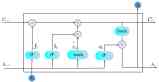
Figure 1. LSTM Structure.
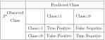
Figure 2. Confusion matrix.
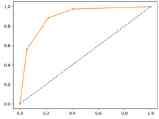
Figure 3. ROC Curve.
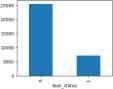
Figure 4. Graphical representation of the loan status variable.
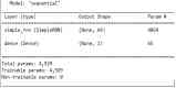
Figure 5. RNN model.
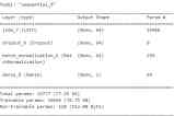
Figure 6. LSTM model.
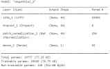
Figure 7. RNN-LSTM Hybrid model.
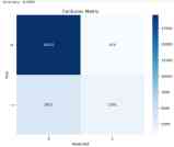
Figure 8. Graphical representation of the loan status variable.
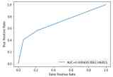
Figure 9. ROC Curve for the RNN-LSTM model.
Information