In this work, we developed a numerical integrator using the Gompertz function model approach with the basic parameters as highlighted by Gompertz in finding and measure the growth in human cells as a basis function involving exponential, logarithmic, and polynomial, hence implemented the numerical integrator to solve problems arising in microbial growth staging. Microbial growth, synonymous to mildew or mold, which is a fungi family commonly found both indoors and outdoors. The indoors occur especially when there is humidity, moisture, oxygen, organic matters and low sunlight. Microbial growth which is the increase in the number of microbial cells which can also be in term of bacterial growth. It can be influenced by various factors to grow including temperature, Water, availability of oxygen, and other nutrient content. The growth staging can be in four phases such as lag, logarithmic, stationary and death phases. A culture of bacterial was taken, the approximate number of strand that was originally present and the growth were calculated using the numerical integration, the results obtained shows a significant, effective and robust improvement on the strand when compared the results with the exact solution. The properties of the integrator were analyzed, considering that Microbial Growth is an increase in the number of bacteria cells in a system when the proper nutrients and environment are provided. Therefore with the approach of Gompertz, the numerical integrator can be applied further to find the growth in each of the phases as they occurs.
| Published in | Applied and Computational Mathematics (Volume 14, Issue 2) |
| DOI | 10.11648/j.acm.20251402.12 |
| Page(s) | 90-100 |
| Creative Commons |
This is an Open Access article, distributed under the terms of the Creative Commons Attribution 4.0 International License (http://creativecommons.org/licenses/by/4.0/), which permits unrestricted use, distribution and reproduction in any medium or format, provided the original work is properly cited. |
| Copyright |
Copyright © The Author(s), 2025. Published by Science Publishing Group |
Numerical Integrator, Gompertz Function, Microbial Growth and Bacteria Cells
XN | EXACT VALUE | NUMERICAL VALUE | ABSOLUTE ERROR |
|---|---|---|---|
[0.00] | [6.900000000000000e+02] | [6.900000000000000e+02] | [0.000000000000000] |
[0.10] | [7.160778840233803e+02] | [7.160797887769264e+02] | [0.001904753546114] |
[0.20] | [7.431416518597050e+02] | [7.431453099924750e+02] | [0.003658132769942] |
[0.30] | [7.712285674083900e+02] | [7.712338211738768e+02] | [0.005253765486827] |
[0.40] | [8.003772966540263e+02] | [8.003839880634949e+02] | [0.006691409468658] |
[0.50] | [8.306279623334798e+02] | [8.306359378448428e+02] | [0.007975511363043] |
[0.60] | [8.620222005488230e+02] | [8.620313143803757e+02] | [0.009113831552668] |
[0.70] | [8.946032192663178e+02] | [8.946133355370953e+02] | [0.010116270777530] |
[0.80] | [9.284158587292990e+02] | [9.284268526788766e+02] | [0.010993949577596] |
[0.90] | [9.635066538705012e+02] | [9.635184124074153e+02] | [0.011758536914158] |
[1.00] | [9.999238988403082e+02] | [9.999363206367847e+02] | [0.012421796476474] |
XN | EXACT VALUE | NUMERICAL VALUE | ABSOLUTE ERROR |
|---|---|---|---|
[1.00] | [9.999238988403082e+02] | [9.999363206367847e+02] | [0.012421796476474] |
[1.10] | [1.037717713779482e+03] | [1.037730709089806e+03] | [0.012995310323049] |
[1.20] | [1.076940113965789e+03] | [1.076953604307765e+03] | [0.013490341976649] |
[1.30] | [1.117645081458867e+03] | [1.117658999268484e+03] | [0.013917809617396] |
[1.40] | [1.159888639359365e+03] | [1.159902927711315e+03] | [0.014288351950654] |
[1.50] | [1.203728928786705e+03] | [1.203743541271387e+03] | [0.014612484682402] |
[1.60] | [1.249226288661646e+03] | [1.249241189529282e+03] | [0.014900867635333] |
[1.70] | [1.296443338345589e+03] | [1.296458503086325e+03] | [0.015164740735827] |
[1.80] | [1.345445063113798e+03] | [1.345460479779864e+03] | [0.015416666066358] |
[1.90] | [1.396298902254159e+03] | [1.396314574157198e+03] | [0.015671903039674] |
[2.00] | [1.449074839057345e+03] | [1.449090790331349e+03] | [0.015951274004237] |
[2.10] | [1.503845490193300e+03] | [1.503861778346467e+03] | [0.016288153166215] |
[2.20] | [1.560686184267167e+03] | [1.560702934185552e+03] | [0.016749918384903] |
[2.30] | [1.619674967396317e+03] | [1.619692503558144e+03] | [0.017536161826911] |
[2.40] | [1.680891364439784e+03] | [1.680911689610851e+03] | [0.020325171067043] |
[2.50] | [1.744426237563714e+03] | [1.744444764708992e+03] | [0.018527145278085] |
[2.60] | [1.810361320250889e+03] | [1.810379186443232e+03] | [0.017866192343490] |
[2.70] | [1.878788232127490e+03] | [1.878805718020890e+03] | [0.017485893399225] |
[2.80] | [1.949801305920745e+03] | [1.949818553207653e+03] | [0.017247286907832] |
[2.90] | [2.023498339839777e+03] | [2.023515445991693e+03] | [0.017106151916323] |
[3.00] | [2.099980799476793e+03] | [2.099997845148666e+03] | [0.017045671873348] |
XN | NUMERICAL VALUE | EXACT VALUE | ABSOLUTE ERROR |
|---|---|---|---|
[0.00] | [7.400000000000000e+02] | [7.400000000000000e+02] | [0.000000000000000] |
[0.10] | [7.611940193364643e+02] | [7.611954714643300e+02] | [0.001452127865718] |
[0.20] | [7.829952571355008e+02] | [7.829980348348699e+02] | [0.002777699369176] |
[0.30] | [8.054211076484687e+02] | [8.054250787591524e+02] | [0.003971110683665] |
[0.40] | [8.284894584619219e+02] | [8.284944899395517e+02] | [0.005031477629814] |
[0.50] | [8.522187059356297e+02] | [8.522246673988334e+02] | [0.005961463203676] |
[0.60] | [8.766277709962579e+02] | [8.766345371543065e+02] | [0.006766158048549] |
[0.70] | [9.017361151942914e+02] | [9.017435673122800e+02] | [0.007452117988578] |
[0.80] | [9.275637569999386e+02] | [9.275717835948619e+02] | [0.008026594923308] |
[0.90] | [9.541312883582614e+02] | [9.541397853114870e+02] | [0.008496953225631] |
[1.00] | [9.814598915475674e+02] | [9.814687617879083e+02] | [0.008870240340912] |
[1.10] | [1.009571356394995e+03] | [1.009580509265756e+03] | [0.009152870760431] |
[1.20] | [1.038488097906053e+03] | [1.038497448286142e+03] | [0.009350380089018] |
[1.30] | [1.068233174366297e+03] | [1.068242641571181e+03] | [0.009467204883777] |
[1.40] | [1.098830305978242e+03] | [1.098839812417671e+03] | [0.009506439429060] |
[1.50] | [1.130303894110867e+03] | [1.130313363617628e+03] | [0.009469506761207] |
[1.60] | [1.162679041272865e+03] | [1.162688396920748e+03] | [0.009355647882330] |
[1.70] | [1.195981571996938e+03] | [1.195990733054317e+03] | [0.009161057378833] |
[1.80] | [1.230238054998969e+03] | [1.230246932316555e+03] | [0.008877317586212] |
[1.90] | [1.265475827418515e+03] | [1.265484315759792e+03] | [0.008488341277143] |
[2.00] | [1.301723023199130e+03] | [1.301730986980392e+03] | [0.007963781261424] |
[2.10] | [1.339008611873735e+03] | [1.339015854532793e+03] | [0.007242659057738] |
[2.20] | [1.377362472291458e+03] | [1.377368654985544e+03] | [0.006182694086192] |
[2.30] | [1.416815649015988e+03] | [1.416819976637718e+03] | [0.004327621729999] |
[2.40] | [1.457403569206754e+03] | [1.457401283914634e+03] | [0.002285292120177] |
[2.50] | [1.499142956754331e+03] | [1.499144942462323e+03] | [0.001985707992390] |
[2.60] | [1.542080660279232e+03] | [1.542084244960776e+03] | [0.003584681543998] |
XN | NUMERICAL VALUE | EXACT VALUE | ABSOLUTE ERROR |
|---|---|---|---|
[2.50] | [1.499142956754331e+03] | [1.499144942462323e+03] | [0.001985707992390] |
[2.60] | [1.542080660279232e+03] | [1.542084244960776e+03] | [0.003584681543998] |
[2.70] | [1.586248878558372e+03] | [1.586253437676532e+03] | [0.004559118159932] |
[2.80] | [1.631682492046569e+03] | [1.631687747775814e+03] | [0.005255729244254] |
[2.90] | [1.678417614250424e+03] | [1.678423411419974e+03] | [0.005797169550533] |
[3.00] | [1.726491460768530e+03] | [1.726497702665671e+03] | [0.006241897141308] |
[3.10] | [1.775942340117185e+03] | [1.775948963192809e+03] | [0.006623075623565] |
[3.20] | [1.826809670957244e+03] | [1.826816632883971e+03] | [0.006961926727172] |
[3.30] | [1.879134007933489e+03] | [1.879141281279721e+03] | [0.007273346232523] |
[3.40] | [1.932957071317150e+03] | [1.932964639934869e+03] | [0.007568617719244] |
[3.50] | [1.988321778832438e+03] | [1.988329635701488e+03] | [0.007856869050784] |
[3.60] | [2.045272279039605e+03] | [2.045280424965263e+03] | [0.008145925657345] |
[3.70] | [2.103853986009496e+03] | [2.103862428862431e+03] | [0.008442852934422] |
[3.80] | [2.164113615173862e+03] | [2.164122369505444e+03] | [0.008754331581258] |
[3.90] | [2.226099220303008e+03] | [2.226108307246215e+03] | [0.009086943206967] |
[4.00] | [2.289860231594508e+03] | [2.289869679006682e+03] | [0.009447412173813] |
[4.10] | [2.355447494872385e+03] | [2.355457337707251e+03] | [0.009842834866049] |
[4.20] | [2.422913311902861e+03] | [2.422923592824576e+03] | [0.010280921714639] |
[4.30] | [2.492311481833677e+03] | [2.492322252111015e+03] | [0.010770277337997] |
[4.40] | [2.563697343759523e+03] | [2.563708664509035e+03] | [0.011320749511924] |
[4.50] | [2.637127820405147e+03] | [2.637139764294787e+03] | [0.011943889640406] |
[4.60] | [2.712661462896397e+03] | [2.712674116486085e+03] | [0.012653589688398] |
[4.70] | [2.790358496550046e+03] | [2.790371963550961e+03] | [0.013467000914716] |
[4.80] | [2.870280867539193e+03] | [2.870295273454084e+03] | [0.014405914890631] |
[4.90] | [2.952492290146399e+03] | [2.952507789079351e+03] | [0.015498932951232] |
[5.00] | [3.037058294018004e+03] | [3.037075079068058e+03] | [0.016785050053841] |
[5.10] | [3.124046270169809e+03] | [3.124064590113213e+03] | [0.018319943404094] |
[5.20] | [3.213525512879304e+03] | [3.213545700751685e+03] | [0.020187872380575] |
[5.30] | [3.305567250164846e+03] | [3.305589776697094e+03] | [0.022526532247866] |
[5.40] | [3.400244641220348e+03] | [3.400270227757587e+03] | [0.025586537239178] |
[5.50] | [3.497632660495767e+03] | [3.497662566383866e+03] | [0.029905888099620] |
[5.60] | [3.597807433386859e+03] | [3.597844467894197e+03] | [0.037034507338376] |
[5.70] | [3.700839388350303e+03] | [3.700895832424399e+03] | [0.056444074095907] |
[5.80] | [3.806869796429933e+03] | [3.806898848652250e+03] | [0.029052222316750] |
[5.90] | [3.915916951661997e+03] | [3.915938059347115e+03] | [0.021107685117386] |
[6.00] | [4.028083883464806e+03] | [4.028100428797081e+03] | [0.016545332275200] |
XN | NUMERICAL VALUE | EXACT VALUE | ABSOLUTE ERROR |
|---|---|---|---|
[0.00] | [7.400000000000000e+02] | [7.400000000000000e+02] | [0.000000000000000] |
[0.10] | [7.611940193364643e+02] | [7.611954714643300e+02] | [0.001452127865718] |
[0.20] | [7.829952571355008e+02] | [7.829980348348699e+02] | [0.002777699369176] |
[0.30] | [8.054211076484687e+02] | [8.054250787591524e+02] | [0.003971110683665] |
[0.40] | [8.284894584619219e+02] | [8.284944899395517e+02] | [0.005031477629814] |
[0.50] | [8.522187059356297e+02] | [8.522246673988334e+02] | [0.005961463203676] |
[0.60] | [8.766277709962579e+02] | [8.766345371543065e+02] | [0.006766158048549] |
[0.70] | [9.017361151942914e+02] | [9.017435673122800e+02] | [0.007452117988578] |
[0.80] | [9.275637569999386e+02] | [9.275717835948619e+02] | [0.008026594923308] |
[0.90] | [9.541312883582614e+02] | [9.541397853114870e+02] | [0.008496953225631] |
[1.00] | [9.814598915475674e+02] | [9.814687617879083e+02] | [0.008870240340912] |
| The Population of Bacteria Cells |
| The Constant Intrinsic Growth of Cells, with |
| The Carrying Capacity of the Growth, That is, the Maximum Size That It Can Achieve with the Available Nutrients |
| [1] | Dennis, G. Z. et al (2013). Differential Equations with Boundary Value Problems. 8th Edition. Brooks/Cole Cengage Learning. Pp 29 - 30. USA. |
| [2] | Fatunla S. O. (1988), Numerical Method for initial value problems of ODEs. Academic Press, San Diego, USA. |
| [3] | Gear, W., (1971). Numerical initial value problems in ODEs, Prentice Hall, Englewood Cliffs, NJ. |
| [4] | Gompertz B. (1860). On one uniform Law of Mortality from Birth to Extreme old age and on the law of sickness. Presented to internal Statistical congress in 1860 and reported in 1871. Journal of the Institute of Actuaries. 16, 329-344. |
| [5] | Henrici, P. (1962). Discrete Variable Methods in ODEs. New York, John Wiley and Sons, USA. |
| [6] | Lambert, J. D. (1962). Numerical Methods for Ordinary Differential Systems. Wiley. New York. |
| [7] | Linda D. B. (2021). Microbial Growth. Biology Libre Texts. Bio.Libretexts.org Oregon State University, USA. |
| [8] | Mehrara E., Forsell A. E., Johanson V., Koolby L., Hultborn R., Bernhardt P. (2013). “A new method to estimate parameters of the growth model for metastatic Tumors.” Theoretical Biology Medical Model. 10: 31-43. |
| [9] | Ogunrinde R. B. and Ayinde S. O. (2017). A Numerical Integration for solving first order differential equation using Gompertz Function Approach. American Journal Computational and Applied Mathematics. 7(6): 143-148. |
| [10] | Uruburu, F. (2003). History and Services of Culture Collections. International Microbiology. 6(2): 101-103. |
| [11] | Sergio, R., Annie, D., and Hubert, M. (2003). “Application of the Gompertz Equation for the study of Xylem Cell Development”. Dendrochronologia. Urban and Fisher Verlag. 21/1: 1-7. ISSN: 1125-7865. |
| [12] | Stoer, J. and Bulirsh, R., (1966). “Numerical Treatment of ODEs by Extrapolation Methods” Numerische Mathematical. 8, 93-104. |
| [13] | Winsor, C. P. (1932). “The Gompertz Curve as a Growth Curve”. Proceedings of the National Academy of Sciences. USA. Vol 18, No1, 1-8. |
| [14] | Zuhaimy, I., Acme, K. and Md-Yunus, J. (2003). “fitting Nonlinear Gompertz curve to Tobacco Growth Data”. Pakistan Journal of Agronomy. 2(4); 223-236. ISSN: 1680-8207. |
| [15] |
Zwietering, M. H. (1990), "Modeling of the Bacterial Growth Curve", Applied and Environmental Microbiology 56 (6): 1875-1881.
https://www.dreamstime.com/stock-photography-fish-feeding-image © 2003-2018. |
APA Style
Olukayode, A. S., John, O. A., Emmanuel, F. S., James, A. K., Micheal, O. O., et al. (2025). Gompertz Function Approach: Numerical Integration for Microbial Growth Problem. Applied and Computational Mathematics, 14(2), 90-100. https://doi.org/10.11648/j.acm.20251402.12
ACS Style
Olukayode, A. S.; John, O. A.; Emmanuel, F. S.; James, A. K.; Micheal, O. O., et al. Gompertz Function Approach: Numerical Integration for Microbial Growth Problem. Appl. Comput. Math. 2025, 14(2), 90-100. doi: 10.11648/j.acm.20251402.12
@article{10.11648/j.acm.20251402.12,
  author = {Ayinde Samuel Olukayode and Omowaye Adeola John and Fadugba Sunday Emmanuel and Adebayo Kayode James and Ogunmiloro Oluwatayo Micheal and Olarinde Oluwakemi Oluwaseun},
  title = {Gompertz Function Approach: Numerical Integration for Microbial Growth Problem},
  journal = {Applied and Computational Mathematics},
  volume = {14},
  number = {2},
  pages = {90-100},
  doi = {10.11648/j.acm.20251402.12},
  url = {https://doi.org/10.11648/j.acm.20251402.12},
  eprint = {https://article.sciencepublishinggroup.com/pdf/10.11648.j.acm.20251402.12},
  abstract = {In this work, we developed a numerical integrator using the Gompertz function model approach with the basic parameters as highlighted by Gompertz in finding and measure the growth in human cells as a basis function involving exponential, logarithmic, and polynomial, hence implemented the numerical integrator to solve problems arising in microbial growth staging. Microbial growth, synonymous to mildew or mold, which is a fungi family commonly found both indoors and outdoors. The indoors occur especially when there is humidity, moisture, oxygen, organic matters and low sunlight. Microbial growth which is the increase in the number of microbial cells which can also be in term of bacterial growth. It can be influenced by various factors to grow including temperature, Water, availability of oxygen, and other nutrient content. The growth staging can be in four phases such as lag, logarithmic, stationary and death phases. A culture of bacterial was taken, the approximate number of strand that was originally present and the growth were calculated using the numerical integration, the results obtained shows a significant, effective and robust improvement on the strand when compared the results with the exact solution. The properties of the integrator were analyzed, considering that Microbial Growth is an increase in the number of bacteria cells in a system when the proper nutrients and environment are provided. Therefore with the approach of Gompertz, the numerical integrator can be applied further to find the growth in each of the phases as they occurs.},
 year = {2025}
}
TY  - JOUR
T1  - Gompertz Function Approach: Numerical Integration for Microbial Growth Problem
AU  - Ayinde Samuel Olukayode
AU  - Omowaye Adeola John
AU  - Fadugba Sunday Emmanuel
AU  - Adebayo Kayode James
AU  - Ogunmiloro Oluwatayo Micheal
AU  - Olarinde Oluwakemi Oluwaseun
Y1  - 2025/03/28
PY  - 2025
N1  - https://doi.org/10.11648/j.acm.20251402.12
DO  - 10.11648/j.acm.20251402.12
T2  - Applied and Computational Mathematics
JF  - Applied and Computational Mathematics
JO  - Applied and Computational Mathematics
SP  - 90
EP  - 100
PB  - Science Publishing Group
SN  - 2328-5613
UR  - https://doi.org/10.11648/j.acm.20251402.12
AB  - In this work, we developed a numerical integrator using the Gompertz function model approach with the basic parameters as highlighted by Gompertz in finding and measure the growth in human cells as a basis function involving exponential, logarithmic, and polynomial, hence implemented the numerical integrator to solve problems arising in microbial growth staging. Microbial growth, synonymous to mildew or mold, which is a fungi family commonly found both indoors and outdoors. The indoors occur especially when there is humidity, moisture, oxygen, organic matters and low sunlight. Microbial growth which is the increase in the number of microbial cells which can also be in term of bacterial growth. It can be influenced by various factors to grow including temperature, Water, availability of oxygen, and other nutrient content. The growth staging can be in four phases such as lag, logarithmic, stationary and death phases. A culture of bacterial was taken, the approximate number of strand that was originally present and the growth were calculated using the numerical integration, the results obtained shows a significant, effective and robust improvement on the strand when compared the results with the exact solution. The properties of the integrator were analyzed, considering that Microbial Growth is an increase in the number of bacteria cells in a system when the proper nutrients and environment are provided. Therefore with the approach of Gompertz, the numerical integrator can be applied further to find the growth in each of the phases as they occurs.
VL  - 14
IS  - 2
ER  -
Mathematics Department, Ekiti State University, Ado Ekiti, Nigeria
Department of Mathematical Sciences, Federal University of Technology, Akure, Nigeria
Mathematics Department, Ekiti State University, Ado Ekiti, Nigeria
Mathematics Department, Ekiti State University, Ado Ekiti, Nigeria
Mathematics Department, Ekiti State University, Ado Ekiti, Nigeria
Mathematics Department, Ekiti State University, Ado Ekiti, Nigeria

Figure 1. The Bar graph analysis of Exact and Numerical Solutions of time (1hour) and 1000 Strands.
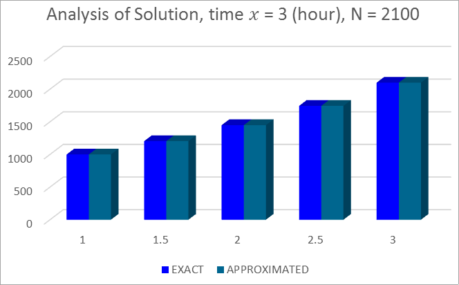
Figure 2. The Bar graph analysis of Exact and Numerical Solutions of time (3hour) and 2100 Strands.
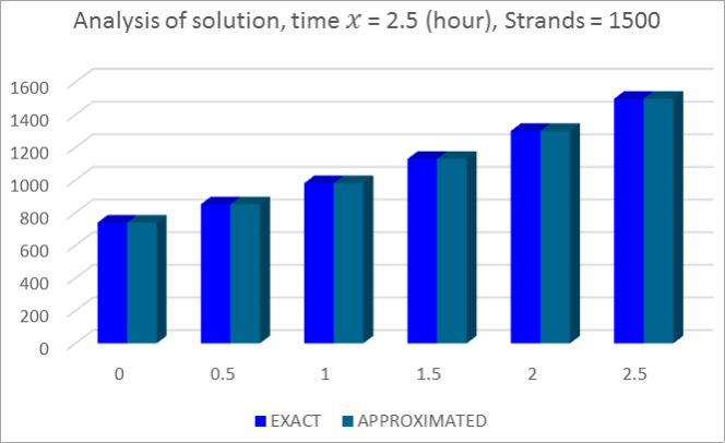
Figure 3. The Bar graph analysis of Exact and Numerical Solutions of time (2.5hour) and 1500 Strands.
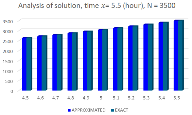
Figure 4. The Bar graph analysis of Exact and Numerical Solutions of time (5.5hour) and 3500 Strands.

Figure 5. The Bar graph analysis of Exact and Numerical Solutions of time (0.0 hour) and 740 Strands.
Information