From Polynomial to Linear Equation to Matrix: The Ezouidi Duality and Second Theorem

Mourad Sultan Ezouidi

doi:doi:10.11648/j.ajaa.20261302.12

Research Article |

| Peer-Reviewed

From Polynomial to Linear Equation to Matrix: The Ezouidi Duality and Second Theorem

Mourad Sultan Ezouidi^*

Published in American Journal of Astronomy and Astrophysics (Volume 13, Issue 2)

Received: 21 April 2026 Accepted: 30 April 2026 Published: 13 May 2026

Views: Downloads:

Download PDF

Share This Article

Twitter
Linked In
Facebook

Abstract

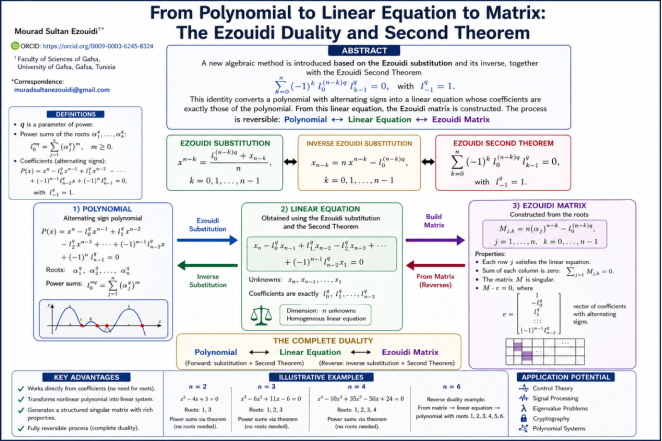
This paper introduces a new algebraic method based on the Ezouidi substitution and its inverse. The Ezouidi substitution expresses powers of the variable in terms of power sums of the roots and new auxiliary variables. A central result is the Ezouidi Second Theorem, an identity that relates power sums of the roots to the polynomial coefficients. The parameter q plays a fundamental role: when q equals zero, the polynomial has a single root repeated n times, giving the binomial form; when q equals one, the polynomial has n roots; when q equals two, the roots are the squares of the original roots; when q equals three, the roots are the cubes; and for higher q, the roots are raised to the corresponding power. Using the Ezouidi substitution together with the Second Theorem, the polynomial is transformed into a linear equation whose coefficients match the original polynomial. From this linear equation we construct the Ezouidi matrix. The matrix is singular, its rows satisfy the linear equation, and its columns sum to zero. The inverse substitution and the Second Theorem reverse the process, recovering the linear equation and the polynomial from the matrix. This establishes a complete triple duality: polynomial, linear equation, and Ezouidi matrix. A detailed example for degree six demonstrates the reverse direction, starting from the matrix to the linear equation and finally to the polynomial. Numerical examples for degrees two, three, and four further confirm the theoretical results. The method provides a new tool for connecting polynomial equations to linear systems and matrix theory.

Published in	American Journal of Astronomy and Astrophysics (Volume 13, Issue 2)
DOI	10.11648/j.ajaa.20261302.12
Page(s)	74-87
Creative Commons	This is an Open Access article, distributed under the terms of the Creative Commons Attribution 4.0 International License (http://creativecommons.org/licenses/by/4.0/), which permits unrestricted use, distribution and reproduction in any medium or format, provided the original work is properly cited.
Copyright	Copyright © The Author(s), 2026. Published by Science Publishing Group

Keywords

Ezouidi Substitution, Inverse Substitution, Ezouidi Second Theorem, Polynomial, Linear Equation, Matrix Duality, Power Sums, Parameter q

1. Introduction

The relationship between polynomial equations and linear systems has long been a subject of interest in algebra and applied mathematics. Classical results such as Vieta's formulas

[2]

connect the coefficients of a polynomial to symmetric functions of its roots, and Newton's identities

[1]

relate power sums to elementary symmetric functions. However, the problem of directly transforming a polynomial into an equivalent linear system remains less explored.

While Newton's identities allow recursive computation of power sums from coefficients, and Viète's formulas relate coefficients to elementary symmetric sums, neither method directly transforms a polynomial into an equivalent linear system. Moreover, Newton's identities require solving a system of equations for higher-degree power sums, and they do not naturally lead to a matrix formulation.

The author has previously explored polynomial resolution methods in a published work

[10]

The connection between polynomial equations and structured matrices has been explored by Mourrain and Pan

[8]

in the multivariate setting. In contrast to their multivariate approach, the present work introduces a fundamentally different univariate method: the Ezouidi substitution, together with the Ezouidi Second Theorem, converts the polynomial directly into a linear equation (LE) whose coefficients are exactly those of the original polynomial. This linear equation then gives rise to the Ezouidi matrix, establishing a triple duality that is absent in classical frameworks.

The Ezouidi substitution is defined as:

x^{n - k} = \frac{l_{0}^{(n - k) q} + x_{n - k}}{n} k = 0, 1, . . ., n - 1

(1)

The inverse Ezouidi substitution is given by:

{x_{n - k} = nx}^{n - k} - l_{0}^{(n - k) q} k = 0, 1, . . ., n - 1

(2)

where

l_{0}^{mq}

denotes the power sum (PS) of the m-th powers of the roots.

The central result of this work is the Second Theorem (Theorem 2), which states that

\sum_{k = 0}^{n} {(- 1)}^{k} l_{0}^{(n - k) q} l_{k - 1}^{q} = 0 with l_{- 1}^{q} = 1

(3)

This identity plays a crucial role in cancelling the nonlinear terms that arise when the Ezouidi substitution is applied to the polynomial.

Using this theorem, we derive a linear equation (LE) satisfied by the roots:

x_{n} - l_{0}^{q} x_{n - 1} + l_{1}^{q} x_{n - 2} - l_{2}^{q} x_{n - 3} {+ l_{3}^{q} x_{n - 4} - l}_{4}^{q} x_{n - 5} +

{l_{5}^{q} x_{n - 6} - l}_{6}^{q} x_{- 7 n} {+ . . . . + (- 1)}^{n - 1} l_{n - 2}^{q} x_{1} = 0

(4)

From this linear equation we construct the Ezouidi matrix M of size n

\times n

, whose entries are

M_{j, k} = n {(α_{j}^{q})}^{(n - k)} - l_{0}^{(n - k) q}

,(5)

where

α_{j}^{q}

are the roots of the polynomial. The matrix is singular, and its rows satisfy the linear equation. In compact form, we have

M ∙ v = 0

,(6)

where

v

is the vector of polynomial coefficients with alternating signs. This establishes a direct duality:

Polynomial ⟷ Linear Equation ⟷ Ezouidi Matrix.

In the sections that follow, each of these three equivalent representations—the polynomial, the linear equation, and the Ezouidi matrix—will be thoroughly examined. Their mutual equivalence will be rigorously established through the Ezouidi substitution, the Second Theorem, and their corresponding inverse transformations.

The paper is organized as follows. Section 2 recalls the standard form of an nth degree polynomial and defines the notation. Section 3 states and proves the Second Theorem. Section 4 presents the Ezouidi substitution and derives the linear equation. Section 5 constructs the Ezouidi matrix and analyses its properties. Section 6 discusses the duality between polynomials, linear equations and matrices. Section 7 provides illustrative examples. Section 8 concludes with remarks and future directions. Polynomial system reductions have been studied by Antoniou and Vologiannidis

[9]

. Algebraic methods for polynomial transformation are discussed by Kumar and Das

[15]

Mourad Sultan Ezouidi is the discoverer of the Ezouidi substitution, the Ezouidi Second Theorem, and the associated duality, and serves as the corresponding author for this work.

2. Standard Form of the Polynomial

Let n be a positive integer. Consider an nth degree polynomial P(x) written in the following alternating sign form:

P(x)=

x^{n} - l_{0}^{q} x^{n - 1} + l_{1}^{q} x^{n - 2} - l_{2}^{q} x^{n - 3} {+ l_{3}^{q} x^{n - 4} - l}_{4}^{q} x^{n - 5}

+ . {+ (- 1)}^{n - 1} l_{n - 2}^{q} x^{1} + {(- 1)}^{n} l_{n - 1}^{q} = 0

(7)

where:

q is a parameter (which may also be interpreted as an index or power.

l_{- 1}^{q} = 1

(coefficient of

x^{n}

l_{0}^{q}, l_{1}^{q}, l_{2}^{q}, l_{3}^{q}, . . . . . . . . l_{n - 1}^{q}

are real or complex coefficients.

The signs alternate strictly, starting with + for

x^{n}

, then −, then +, etc.

2.1. Roots of the Polynomial

Let the roots of P(x) be denoted by

α_{1}^{q}

α_{2}^{q}

α_{3}^{q}

,……..,

α_{n}^{q}

. By the fundamental theorem of algebra, we have

P (x) = \prod_{j = 1}^{n} (x - α_{j}^{q})

(8)

2.2. Power Sums

For any integer

m \geq 1

, define the power sum of the roots as

l_{0}^{mq} = \sum_{j = 1}^{n} {(α_{j}^{q})}^{m}

.(9)

For a detailed treatment of symmetric functions and power sums, see Macdonald

[3]

New power sum identities have been developed by Lee, Park, and Kim

[13]

In particular:

l_{0}^{q} = n

(sum of the 0th powers, i.e., number of roots),

l_{0}^{q} = \sum_{j = 1}^{n} α_{j}^{q} (10) l_{0}^{2 q} = \sum_{j = 1}^{n} {(α_{j}^{q})}^{2}

(11)

and so on.

These power sums will appear naturally in the Ezouidi substitution and the Second Theorem.

2.3. Confficient Vector

Define the vector of coefficients (with alternating signs) as:

v = [\begin{matrix} \begin{matrix} 1 \\ {- l}_{0}^{q} \\ l_{1}^{q} \end{matrix} \\ \begin{matrix} {- l}_{2}^{q} \\ l_{3}^{q} \\ ⋮ \end{matrix} \\ {(- 1)}^{n - 1} l_{n - 2}^{q} \end{matrix}]

(12)

This vector will play a central role in the matrix formulation.

For a modern introduction to linear algebra, see Woerdeman

[7]

3. The Second Theorem – Statement and Proof

Theorem 2 (Second Theorem – Ezouidi)

For any integer

n \geq 1

let

l_{0}^{mq}

be the power sum of the roots of an nth degree polynomial, and let

l_{k - 1}^{q}

be the polynomial coefficients with

l_{- 1}^{q} = 1

. Then the following identity holds:

\sum_{k = 0}^{n} {(- 1)}^{k} l_{0}^{(n - k) q} l_{k - 1}^{q} = 0,

with

l_{- 1}^{q} = 1

(13)

Explicit expanded form:

l_{0}^{nq} - l_{0}^{q} l_{0}^{(n - 1) q} + l_{1}^{q} l_{0}^{(n - 2) q} - l_{2}^{q} l_{0}^{(n - 3) q} + l_{3}^{q} l_{0}^{(n - 4) q} + . . . + {(- 1)}^{n - 1} l_{n - 2}^{q} l_{0}^{q} + n {(- 1)}^{n} l_{n - 1}^{q} = 0

(14)

Proof (Direct verification at q=0)

Set q=0. Then:

l_{0}^{0} = n

l_{k - 1}^{q} = c_{n}^{k - 1 + 1} = c_{n}^{k}

(binomial coefficients).

The left-hand side becomes:

\sum_{k = 0}^{n} {(- 1)}^{k} n c_{n}^{k} = n \sum_{k = 0}^{n} {(- 1)}^{k} c_{n}^{k}

(15)

By the binomial theorem:

\sum_{k = 0}^{n} {(- 1)}^{k} c_{n}^{k} = {(1 - 1)}^{n} = 0

(16)

The binomial theorem used in this proof can be found in standard references such as Graham, Knuth, and Patashnik

[6]

Thus the sum equals 0 and the theorem holds at q=0.

4. Ezouidi Substitution and Derivation of the Linear Equation

We define the Ezouidi substitution as follows: for k=0,1,2,…….,n-1,

x^{n - k} = \frac{l_{0}^{(n - k) q} + x_{n - k}}{n}

(17)

where:

x^{n - k}

is the power of x in the polynomial.

l_{0}^{(n - k) q}

is the power sum of the roots, as defined in Section 2.

x_{n - k}

is a new variable (which will become the unknown in the linear equation).

n is the degree of the polynomial.

For k=n, we have

x^{0} = 1

(no substitution).

4.1. Derivation of the Linear Equation

Start with the polynomial equation P(x)=0, where

P(x)=

x^{n} - l_{0}^{q} x^{n - 1} + l_{1}^{q} x^{n - 2} - l_{2}^{q} x^{n - 3} {+ l_{3}^{q} x^{n - 4} - l}_{4}^{q} x^{n - 5} + . {+ (- 1)}^{n - 1} l_{n - 2}^{q} x^{1} + {(- 1)}^{n} l_{n - 1}^{q} = 0

(18)

P (x) = \sum_{k = 0}^{n} {(- 1)}^{k} l_{k - 1}^{q} x^{n - k} = \sum_{k = 0}^{n - 1} {(- 1)}^{k} l_{k - 1}^{q} x^{n - k} + {(- 1)}^{n} l_{n - 1}^{q} = 0

(19)

Substitute the Ezouidi substitution for each

x^{n - k}

P (x) = \sum_{k = 0}^{n - 1} {(- 1)}^{k} l_{k - 1}^{q} \frac{l_{0}^{(n - k) q} + x_{n - k}}{n} + {(- 1)}^{n} l_{n - 1}^{q} = 0

(20)

Separate the sum into two parts:

P (x) = \sum_{k = 0}^{n - 1} {(- 1)}^{k} l_{k - 1}^{q} (\frac{l_{0}^{(n - k) q}}{n}) + \sum_{k = 0}^{n - 1} {(- 1)}^{k} l_{k - 1}^{q} (\frac{x_{n - k}}{n}) + {(- 1)}^{n} l_{n - 1}^{q} = 0

(21)

P (x) = \frac{1}{n} \sum_{k = 0}^{n - 1} {(- 1)}^{k} l_{k - 1}^{q} l_{0}^{(n - k) q} + \frac{1}{n} \sum_{k = 0}^{n - 1} {(- 1)}^{k} l_{k - 1}^{q} x_{n - k} + {(- 1)}^{n} l_{n - 1}^{q} = 0

(22)

4.2. Use of the Second Theorem

The Second Theorem (proved in Section 3) states that

\sum_{k = 0}^{n} {(- 1)}^{k} l_{0}^{(n - k) q} l_{k - 1}^{q} = 0 with l_{- 1}^{q} = 1

(23)

Separating the last term (k=n) gives

\sum_{k = 0}^{n - 1} {(- 1)}^{k} l_{0}^{(n - k) q} l_{k - 1}^{q} + {(- 1)}^{n} {nl}_{n - 1}^{q} = 0

(24)

since

l_{0}^{0} = n .

Therefore,

\sum_{k = 0}^{n - 1} {(- 1)}^{k} l_{0}^{(n - k) q} l_{k - 1}^{q} = - {(- 1)}^{n} n l_{n - 1}^{q}

(25)

Substituting this into the expression for P(x):

P (x) = \frac{1}{n} {(- (- 1)}^{n} n l_{n - 1}^{q}) + \frac{1}{n} \sum_{k = 0}^{n - 1} {(- 1)}^{k} l_{k - 1}^{q} x_{n - k} + {(- 1)}^{n} l_{n - 1}^{q} = 0

(26)

The first and third terms cancel:

- {(- 1)}^{n} l_{n - 1}^{q} + {(- 1)}^{n} l_{n - 1}^{q} = 0

(27)

Thus,

\frac{1}{n} \sum_{k = 0}^{n - 1} {(- 1)}^{k} l_{k - 1}^{q} x_{n - k} = 0

(28)

Since P(x)=0, we obtain the linear equation:

\sum_{k = 0}^{n - 1} {(- 1)}^{k} l_{k - 1}^{q} x_{n - k} = 0

(29)

4.3. Explicit Form of the Linear Equation

Writing the sum explicitly gives

x_{n} - l_{0}^{q} x_{n - 1} + l_{1}^{q} x_{n - 2} - l_{2}^{q} x_{n - 3} {+ l_{3}^{q} x_{n - 4} - l}_{4}^{q} x_{n - 5} + {l_{5}^{q} x_{n - 6} - l}_{6}^{q} x_{- 7 n} {+ . . . . + (- 1)}^{n - 1} l_{n - 2}^{q} x^{1} = 0

(30)

This is a linear equation in the n unknowns

x_{n}, x_{n - 1}, x_{n - 2}, x_{n - 3}, . . . . . . . . . x_{1}

5. Construction of the Ezouidi Matrix

From the linear equation derived in Section 4:

x_{n} - l_{0}^{q} x_{n - 1} + l_{1}^{q} x_{n - 2} - l_{2}^{q} x_{n - 3} {+ l_{3}^{q} x_{n - 4} - l}_{4}^{q} x_{n - 5} + {l_{5}^{q} x_{n - 6} - l}_{6}^{q} x_{- 7 n} {+ . . . . + (- 1)}^{n - 1} l_{n - 2}^{q} x^{1} = 0

(31)

we construct the Ezouidi matrix M of size

n \times n

5.1. Definition

For each root

α_{j}^{q}

of the polynomial, define the entries of M as:

M_{j, k} = n {(α_{j}^{q})}^{(n - k)} - l_{0}^{(n - k) q}

,(32)

where:

J=1,2,….,n (row index, corresponding to the root

α_{j}^{q}

k=0,1,2…,n-1 (column index, corresponding to the power n-k),

l_{0}^{(n - k) q} = \sum_{k = 1}^{n} {(α_{j}^{q})}^{n - k}

is the power sum.(33)

Explicit Matrix Form

M = [\begin{matrix} n {{(α}_{1}^{q})}^{n} - l_{0}^{nq} & n {{(α}_{1}^{q})}^{n - 1} - l_{0}^{(n - 1) q} & n {{(α}_{1}^{q})}^{2} - l_{0}^{2 q} . . . n {{(α}_{1}^{q})}^{1} - l_{0}^{q} \\ n {{(α}_{2}^{q})}^{n} - l_{0}^{nq} & n {{(α}_{2}^{q})}^{n - 1} - l_{0}^{(n - 1) q} & n {{(α}_{2}^{q})}^{2} - l_{0}^{2 q} . . . n {{(α}_{2}^{q})}^{1} - l_{0}^{q} \\ \begin{matrix} ⋮ \\ n {{(α}_{n}^{q})}^{n} - l_{0}^{nq} \end{matrix} & \begin{matrix} ⋮ \\ n {{(α}_{n}^{q})}^{n - 1} - l_{0}^{(n - 1) q} \end{matrix} & \begin{matrix} \begin{matrix} ⋮ & ⋱ \end{matrix} \\ n {{(α}_{n}^{q})}^{2} - l_{0}^{2 q} . . . n {{(α}_{n}^{q})}^{1} - l_{0}^{q} \end{matrix} \end{matrix}]

(34)

5.2. Properties of the Ezouidi Matrix

Rows are the roots of the linear equation:

Each row j of M corresponds to a root

α_{j}^{q}

and satisfies the linear equation:

\sum_{j = 0}^{n} M_{j, k} = 0

for each k(35)

Sum of each column is zero:

For any fixed column k, summing over all rows j gives:

\sum_{j = 0}^{n} M_{j, k} = \sum_{j = 0}^{n} (n {(α_{j}^{q})}^{(n - k)} - l_{0}^{(n - k) q}) = n l_{0}^{(n - k) q} - n l_{0}^{(n - k) q} = 0

(36)

Column sum: The sum of all entries in any column is zero:

\sum_{j = 0}^{n} M_{j, k} = 0

for each k(37)

Singularity and Nullspace: Since the columns sum to zero, the columns are linearly dependent, hence detM=0 and the vector vsatisfies

M ∙ v = 0

(38).

Thus

v

is in the nullspace of M.

v = [\begin{matrix} \begin{matrix} 1 \\ {- l}_{0}^{q} \\ l_{1}^{q} \end{matrix} \\ \begin{matrix} {- l}_{2}^{q} \\ l_{3}^{q} \\ ⋮ \end{matrix} \\ {(- 1)}^{n - 1} l_{n - 2}^{q} \end{matrix}]

(39)

The singularity and nullspace properties of the Ezouidi matrix are related to standard results in matrix analysis

[4]

. Numerical aspects of matrix computations are discussed in Golub and Van Loan

[5]

5.3. Duality

The Ezouidi matrix establishes a direct correspondence:

Polynomial ⟷ Linear Equation ⟷ Ezouidi Matrix.

This duality allows one to move freely between these three representations, using the Ezouidi substitution and its inverse.

The present work is related to modern studies on polynomial-matrix transformations

[11]

, duality in linear algebra

[12]

, and matrix methods for polynomial root finding

[14]

5.4. Summary

Rows of M = roots of the linear equation.

Columns of M sum to zero.

The matrix is singular.

The coefficient vector v is a nullspace vector.

Download: Download full-size image

Figure 1. Ezouidi duality: Polynomial ↔ Linear Equation ↔ Ezouidi Matrix, using the Ezouidi substitution, inverse substitution, and the Second Theorem.

6. From Matrix to Linear Equation to Polynomial (Reverse Duality)

In this section, we reverse the direction. We start from the Ezouidi matrix and recover first the linear equation, then the original polynomial.

Step 1: Recall the Ezouidi matrix and the vector v

From Section 5, the Ezouidi matrix M is defined by:

M_{j, k} = n {(α_{j}^{q})}^{(n - k)} - l_{0}^{(n - k) q}

,(40)

The vector v (coefficients with alternating signs) is: j=1,2,…..,n and k=0,1,2….,n-1

v = [\begin{matrix} \begin{matrix} 1 \\ {- l}_{0}^{q} \\ l_{1}^{q} \end{matrix} \\ \begin{matrix} {- l}_{2}^{q} \\ l_{3}^{q} \\ ⋮ \end{matrix} \\ {(- 1)}^{n - 1} l_{n - 2}^{q} \end{matrix}]

(41)

We also know from Section 5 that:

M ∙ v = 0

(42)

Step 2: From

M ∙ v = 0

to the linear equation

Take the first row of

M ∙ v = 0

(43)

(any row works, since all rows satisfy the same relation). This gives:

(

n {(α_{j}^{q})}^{n} - l_{0}^{nq}) . 1 - l_{0}^{q} (n {(α_{j}^{q})}^{(n - 1)} - l_{0}^{(n - 1) q}) + l_{1}^{q} (n {(α_{j}^{q})}^{(n - 2)} - l_{0}^{(n - 2) q}) + . . . . . . . . +

{(- 1)}^{n - 2} l_{n - 3}^{q} (n {(α_{j}^{q})}^{2} - l_{0}^{2 q}) + {(- 1)}^{n - 1} l_{n - 2}^{q} (n {(α_{j}^{q})}^{1} - l_{0}^{)}) = 0

(44)

Now we use the inverse Ezouidi substitution, which we introduced earlier:

x_{n - k} = n {(α_{j}^{q})}^{(n - k)} - l_{0}^{(n - k) q}

,(45)

Thus, the terms

n {(α_{j}^{q})}^{(n - k)} - l_{0}^{(n - k) q}

, become simply

x_{n - k}

Substituting these into the equation, we obtain:

x_{n} (1) - {x_{n - 1} (l}_{0}^{q}) + {x_{n - 2} (l}_{1}^{q}) - {x_{n - 3} (l}_{2}^{q}) +

{x_{n - 4} (l}_{3}^{q}) + . . . . . + x_{1} {(- 1)}^{n - 1} l_{n - 2}^{q} = 0

(46)

This is exactly the linear equation we derived in Section 4

x_{n} - l_{0}^{q} x_{n - 1} + l_{1}^{q} x_{n - 1} - l_{2}^{q} {x_{n - 3} + l}_{3}^{q} {x_{n - 4} - x_{n - 5} l}_{4}^{q}

+ . . . . . + {(- 1)}^{n - 1} l_{n - 2}^{q} x_{1} = 0

(47)

Step 3: From the linear equation to the polynomial

Now we reverse the process of Section 4 (where the linear equation was derived).

Starting from the linear equation:

x_{n} - l_{0}^{q} x_{n - 1} + l_{1}^{q} x_{n - 1}

- l_{2}^{q} {x_{n - 3} + l}_{3}^{q} {x_{n - 4} - x_{n - 5} l}_{4}^{q} + . . . . . + {(- 1)}^{n - 1} l_{n - 2}^{q} x_{1} = 0

(48)

We apply the inverse substitution in the opposite direction. Recall that:

x_{n - k}

n x^{(n - k)} - l_{0}^{(n - k) q}

(49)

Substitute this into the linear equation. For a given root

α_{j}^{q}

, we have

x^{n - k} = {(α_{j}^{q})}^{n - k}

(50). Then

n x^{n} - l_{0}^{nq} - l_{0}^{q} (n x^{(n - 1)} - l_{0}^{(n - 1) q}) + l_{1}^{q} (n x^{(n - 2)} - l_{0}^{(n - 2) q}) - l_{2}^{q} (n x^{(n - 3)} - l_{0}^{(n - 3) q})

+ . . . + {(- 1)}^{n - 1} l_{n - 2}^{q} (n x^{1} - l_{0}^{q}) = 0

(51)

Separate the terms as before:

n {α_{j}^{q}}^{n} - {nl}_{0}^{q} {α_{j}^{q}}^{(n - 1)} + n l_{1}^{q} {α_{j}^{q}}^{(n - 2)} - n l_{2}^{q} {α_{j}^{q}}^{(n - 3)} + \dots + {(- 1)}^{n - 1} n l_{n - 2}^{q} {α_{j}^{q}}^{1} - l_{0}^{nq} - l_{0}^{q} l_{0}^{(n - 1) q} + l_{1}^{q} l_{0}^{(n - 2) q}

+ . . + - {(- 1)}^{n - 1} l_{n - 2}^{q} l_{0}^{q} = 0

(52)

The second bracket is almost the Second Theorem, missing the last term. Using the Second Theorem (proved in Section 3), we have:

l_{0}^{nq} - l_{0}^{q} l_{0}^{(n - 1) q} + l_{1}^{q} l_{0}^{(n - 2) q} - l_{2}^{q} l_{0}^{(n - 3) q} +

l_{3}^{q} l_{0}^{(n - 4) q} . + . . . + {(- 1)}^{n - 1} l_{n - 2}^{q} l_{0}^{q} = (- {(- 1)}^{n} n l_{n - 1}^{q})

(53)

I.e

\sum_{k = 0}^{n - 1} {(- 1)}^{k} l_{0}^{(n - k) q} l_{k - 1}^{q} + {(- 1)}^{n} l_{n - 1}^{q} = 0,

with

l_{- 1}^{q} = 1

(54)

Substitute this into the equation:

n {α_{j}^{q}}^{n} - {nl}_{0}^{q} {α_{j}^{q}}^{(n - 1)} + n l_{1}^{q} {α_{j}^{q}}^{(n - 2)} - n l_{2}^{q} {α_{j}^{q}}^{(n - 3)}

+ . . . + {(- 1)}^{n - 1} n l_{n - 2}^{q} {α_{j}^{q}}^{1} - (- {(- 1)}^{n} n l_{n - 1}^{q}) = 0

(55)

That is:

n {(α}_{j}^{q}^{n} - l_{0}^{q} {α_{j}^{q}}^{(n - 1)} + l_{1}^{q} {α_{j}^{q}}^{(n - 2)} -

l_{2}^{q} {α_{j}^{q}}^{(n - 3)} + . . . + {(- 1)}^{n - 1} l_{n - 2}^{q} {α_{j}^{q}}^{1} + {(- 1)}^{n} n l_{n - 1}^{q} = 0

(56)

Divide by n (since n

\neq

{α_{j}^{q}}^{n} - l_{0}^{q} {α_{j}^{q}}^{(n - 1)} + l_{1}^{q} {α_{j}^{q}}^{(n - 2)} -

l_{2}^{q} {α_{j}^{q}}^{(n - 3)} + . . . + {(- 1)}^{n - 1} l_{n - 2}^{q} {α_{j}^{q}}^{1} + {(- 1)}^{n} l_{n - 1}^{q} = 0

(57)

This is exactly P(

α_{j}^{q}

)=0. Therefore, the

α_{j}^{q}

are the roots of the polynomial:

x^{n} - l_{0}^{q} x^{(n - 1)} + l_{1}^{q} x^{(n - 2)} -

l_{2}^{q} x^{(n - 3)} + . . . + {(- 1)}^{n - 1} l_{n - 2}^{q} x^{1} + {(- 1)}^{n} l_{n - 1}^{q} = 0

(58)

Step 4: Conclusion of the reverse duality

We have shown:

Ezouidi Matrix

\begin{matrix} M ∙ v = 0 \\ \to \end{matrix}

Linear Equation

\begin{matrix} Inverse Substitution + Second Theorem \\ \to \end{matrix}

Polynomial

Together with Sections 3–5, this completes the full duality:

Polynomial ⟷ Linear Equation ⟷ Ezouidi Matrix.

7. Illustrative Examples

We now illustrate the Ezouidi method with concrete numerical examples for degrees n=2,3,4,6

7.1. Example 1: n=2

Polynomial

Consider the polynomial

P(x)=

x^{2} - 4 x + 3 = 0

,(59)

Roots (Given for Verification Only)

The roots are:

α_{1} = 1, α_{2} = 3

These are provided only to verify the classical method. They are not needed for the Ezouidi method.

Coefficients

In the standard alternating sign form

P(x)=

x^{n} - l_{0}^{q} x^{n - 1} + l_{1}^{q} x^{n - 2} - l_{2}^{q} x^{n - 3} +

l_{3}^{q} x^{n - 4} + . . + {(- 1)}^{n} l_{n - 1}^{q}

(60)

For n=2

P (x) = x^{2} - l_{0}^{q} x^{1} + l_{1}^{q} = 0

(61)

Comparing with

x^{2} - 4 x^{1} + 3 = 0

(62)

l_{- 1}^{q} = 1, l_{0}^{q} = 4, l_{1}^{q} = 3

Classical Method (Requires Roots)

To find power sums using classical algebra, you must know the roots.

First power sum (sum of roots):

l_{0}^{q} = 1 + 3 = 4

(63)

Second power sum (sum of squares of roots):

{l_{0}^{2 q} = α_{1}}^{2} + {α_{2}}^{2} = 1^{2} + 3^{2} = 1 + 9 = 10

(64)

Limitation: Without the roots, classical methods cannot find

l_{0}^{2 q}

The Ezouidi Second Theorem (n = 2)

For n = 2, the Ezouidi Second Theorem states:

\sum_{k = 0}^{2} {(- 1)}^{k} l_{0}^{(2 - k) q} l_{k - 1}^{q} = l_{0}^{2 q} - {(l_{0}^{q})}^{2} + 2 l_{1}^{q}

(65)

Table 1. Second Theorem terms for n=2.

k	Term	Result
For k=0	${(- 1)}^{0} l_{0}^{(2) q} l_{- 1}^{q}$	$l_{0}^{2 q}$
For k=1	${(- 1)}^{1} l_{0}^{q} l_{0}^{q}$	$- {(l_{0}^{q})}^{2}$
For k=2	${(- 1)}^{2} l_{0}^{(0) q} l_{1}^{q}$	$2 l_{1}^{q}$ (since $l_{0}^{0}$ =n=2)

Therefore:

\sum_{k = 0}^{2} {(- 1)}^{k} l_{0}^{(2 - k) q} l_{k - 1}^{q} = l_{0}^{2 q} - {(l_{0}^{q})}^{2} + 2 l_{1}^{q} = 0

(66)

Using the theorem to find

l_{0}^{2 q}

without roots

From the theorem equation, solve for

l_{0}^{2 q}

l_{0}^{2 q} - {(l_{0}^{q})}^{2} + 2 l_{1}^{q} = 0

(67)

Now substitute the coefficients (read directly from the polynomial in Section 2):

l_{0}^{q} = 1 + 3 = 4

(68)

l_{0}^{2 q} = {(l_{0}^{q})}^{2} - 2 l_{1}^{q} = 4^{2} - 2 (3) = 16 - 6 = 10

(69)

We found

l_{0}^{2 q} = 10

without ever using the roots 1 and 3!

Verification That the Theorem Holds

Plug the values back into the theorem equation:

\sum_{k = 0}^{2} {(- 1)}^{k} l_{0}^{(2 - k) q} l_{k - 1}^{q} = l_{0}^{2 q} - {(l_{0}^{q})}^{2} + 2 l_{1}^{q} = 10 - 16 + 6 = 0

✓(70)

The theorem is satisfied.

Applying the Ezouidi Substitution to Get the Linear Equation

The inverse Ezouidi substitution is:

x^{2 - k} = \frac{l_{0}^{(2 - k) q} + x_{2 - k}}{2}

, k=0,1(71)

Substitute into P(x)=0(72)

\frac{l_{0}^{2 q} + x_{2}}{2} - 4 \frac{l_{0}^{q} + x_{1}}{2} + 3 = 0

(73)

Multiply by 2

l_{0}^{2 q} + x_{2}

-4(

l_{0}^{q} + x_{1}

)+6=0(74)

Expand

x_{2} - 4 x_{1}

[l_{0}^{2 q} - 4 l_{0}^{q} + 6] = 0

(75)

Evaluate the bracket using

l_{0}^{2 q} = 10

and

l_{0}^{q} = 4

l_{0}^{2 q} - 4 l_{0}^{q} + 6 = 10 - 16 + 6 = 0

(76)

Therefore, the linear equation is:

x_{2} - 4 x_{1} = 0

.(77).

Constructing the Ezouidi Matrix and Verification

M ∙ v = 0

(78)

Ezouidi Matrix:

M_{j, k} = n {(α_{j}^{q})}^{(n - k)} - l_{0}^{(n - k) q}

,(79)

The Ezouidi matrix is:

M = [\begin{matrix} 2 ({1)}^{2} - 10 & 2 ({1)}^{1} - 4 \\ 2 ({3)}^{2} - 10 & 2 ({3)}^{1} - 4 \end{matrix}] = [\begin{matrix} - 8 & - 2 \\ 8 & 2 \end{matrix}]

(80)

Each row satisfies

x_{2} - 4 x_{1} = 0

(81)

Row 1:(−8)−4(−2)=0(−8)−4(−2)=0(82)

Row 2:8−4(2)=08−4(2)=0.(83)

The vectorv=

[\begin{matrix} 1 \\ - 4 \end{matrix}]

satisfies

M ∙ v = 0

(84).

The polynomial is recovered as

x^{2} - 4 x + 3 = 0

.(85)

Compare Classical vs. Ezouidi

Table 2. Comparison of Classical and Ezouidi methods for n=2.

Aspect	Classical Method	Ezouidi Method
Requires roots?	✅ Yes ( $α_{1} = 1, α_{2} = 3$ )	❌ No
Requires only coefficients?	❌ No	✅ Yes ( $l_{0}^{q} = 4, l_{1}^{q} = 3$
Formula used	$l_{0}^{2 q} = 1^{2} + 3^{2} = 10$	$l_{0}^{2 q} = {{(l}_{0}^{q})}^{2} - 2 l_{1}^{q}$
Result	$l_{0}^{2 q}$ =10	$l_{0}^{2 q} = 10$

Conclusion: Both methods yield the same result. However, the classical method requires knowing the roots first, while the Ezouidi method works directly from the coefficients. This demonstrates the power of the Ezouidi Second Theorem.

7.2. Example 2: n=3

Polynomial

Consider the polynomial

P(x)=

{x^{3} - 6 x}^{2} + 11 x^{} - 6 = 0

,(86)

Roots (Given for Verification Only)

The roots are:

α_{1} = 1, α_{2} = 2, α_{3} = 3

These are provided only to verify the classical method. They are not needed for the Ezouidi method.

Coefficients

In the standard alternating sign form

P(x)=

x^{n} - l_{0}^{q} x^{n - 1} + l_{1}^{q} x^{n - 2} - l_{2}^{q} x^{n - 3} +

l_{3}^{q} x^{n - 4} + . . + {(- 1)}^{n} l_{n - 1}^{q}

(87)

For n=3

P (x) = x^{3} - l_{0}^{q} x^{2} + l_{1}^{q} x^{1} - l_{2}^{q} = 0

(88)

Comparing with

x^{3} - 6 x^{2} + 11 x^{1} - 6 = 0

(89)

l_{- 1}^{q} = 1, l_{0}^{q} = 6, l_{1}^{q} = 11, l_{2}^{q} = 6

Classical Method (Requires Roots)

To find power sums using classical algebra, you must know the roots.

First power sum (sum of roots):

l_{0}^{q} = 1 + 2 + 3 = 6

(90)

Second power sum (sum of squares of roots):

l_{0}^{2 q} = {α_{1}}^{2} + {α_{2}}^{2} + {α_{3}}^{2} = 1^{2} + 2^{2} + 3^{2} = 1 + 4 + 9 = 14

(91)

l_{0}^{3 q} = {α_{1}}^{3} + {α_{2}}^{3} + {α_{3}}^{3} = 1^{3} + 2^{3} + 3^{3} = 1 + 8 + 27 = 36

(92)

Limitation: Without the roots, classical methods cannot find

l_{0}^{2 q}

and

l_{0}^{3 q}

The Ezouidi Second Theorem (n = 3)

For n = 3, the Ezouidi Second Theorem states:

\sum_{k = 0}^{3} {(- 1)}^{k} l_{0}^{(3 - k) q} l_{k - 1}^{q} = l_{0}^{3 q} - l_{0}^{2 q} l_{0}^{q} + l_{1}^{q} l_{0}^{q} - 3 l_{2}^{q}

(93)

Table 3. Second Theorem terms for n=3.

k	Term	Result
For k=0	${(- 1)}^{0} l_{0}^{(3) q} l_{- 1}^{q}$	$l_{0}^{3 q}$
For k=1	${(- 1)}^{1} l_{0}^{2 q} l_{0}^{q}$	$- l_{0}^{2 q} l_{0}^{q}$
For k=2	${(- 1)}^{2} l_{0}^{q} l_{1}^{q}$	$l_{0}^{q} l_{1}^{q}$
For k=3	${{(- 1)}^{1} l}_{0}^{0} l_{2}^{q}$	$- 3 l_{2}^{q}$ (since $l_{0}^{0}$ =n=3)

Therefore:

\sum_{k = 0}^{3} {(- 1)}^{k} l_{0}^{(3 - k) q} l_{k - 1}^{q} = l_{0}^{3 q} - l_{0}^{2 q} l_{0}^{q} + l_{1}^{q} l_{0}^{q} - 3 l_{2}^{q} = 0

(94)

Using the theorem to find

l_{0}^{2 q}

and

l_{0}^{3 q}

without roots

From the theorem equation, solve for

l_{0}^{2 q}

and

l_{0}^{3 q}

l_{0}^{2 q} - {(l_{0}^{q})}^{2} + 2 l_{1}^{q} = 0

(95)

Now substitute the coefficients (read directly from the polynomial in Section 2):

l_{0}^{q} = 1 + 2 + 3 = 6

(96)

l_{0}^{2 q} = {(l_{0}^{q})}^{2} - 2 l_{1}^{q} = 6^{2} - 2 (11) = 36 - 22 = 14

(97)

l_{0}^{3 q} - l_{0}^{3 q} l_{0}^{q} + l_{1}^{q} l_{0}^{q} - 3 l_{2}^{q} = 0

(98)

Now substitute the coefficients (read directly from the polynomial in Section 2,

l_{0}^{2 q} = 14)

l_{0}^{3 q} = l_{0}^{2 q} l_{0}^{q} - l_{1}^{q} l_{0}^{q} + 3 l_{2}^{q} = 14 (6) - 11 (6) + 3 (6) = 84 - 66 + 18 = 36

(99)

We found

l_{0}^{2 q} = 14

and

l_{0}^{3 q} = 36

without ever using the roots 1,2 and 3!

Verification That the Theorem Holds

Plug the values back into the theorem equation:

\sum_{k = 0}^{3} {(- 1)}^{k} l_{0}^{(3 - k) q} l_{k - 1}^{q} = l_{0}^{3 q} - l_{0}^{3 q} l_{0}^{q} + l_{1}^{q} l_{0}^{q} - 3 l_{2}^{q} =

14 (6) - 11 (6) - 3 (6) = 84 - 84 = 0

✓(100)

The theorem is satisfied.

Applying the Ezouidi Substitution to Get the Linear Equation

The inverse Ezouidi substitution is:

x^{3 - k} = \frac{l_{0}^{(3 - k) q} + x_{3 - k}}{3}

, k=0,1,2(101)

Substitute into P(x)=0(102)

\frac{l_{0}^{3 q} + x_{3}}{3} - 6 \frac{l_{0}^{2 q} + x_{2}}{3} + 11 \frac{l_{0}^{q} + x_{1}}{3} - 6 = 0

(103)

Multiply by 3

l_{0}^{3 q} + x_{3} - 6

(

l_{0}^{2 q} + x_{2}) + 11 (l_{0}^{q} + x_{1}) - 18

=0(104)

Expand

x_{3} - 6 x_{2} + 11 x_{1}

[l_{0}^{3 q} - 6 l_{0}^{2 q} + 11 l_{0}^{q} - 18] = 0

(105)

Evaluate the bracket using

l_{0}^{3 q} = 36, l_{0}^{2 q} = 14

and

l_{0}^{q} = 6

l_{0}^{3 q} - 6 l_{0}^{2 q} + 11 l_{0}^{q} - 18 = 36 - 6 (14) + 11 (6) =

36 - 84 + 66 - 18 = 0

(106)

Therefore, the linear equation is:

x_{3} - 6 x_{2} + 11 x_{1} = 0

.(107).

Constructing the Ezouidi Matrix and Verification

M ∙ v = 0

(108)

Ezouidi Matrix:

M_{j, k} = n {(α_{j}^{q})}^{(n - k)} - l_{0}^{(n - k) q}

,(109)

The Ezouidi matrix is:

M = [\begin{matrix} 3 ({1)}^{3} - 36 & \begin{matrix} 3 ({1)}^{2} - 14 & 3 ({1)}^{1} - 6 \end{matrix} \\ \begin{matrix} 3 ({2)}^{3} - 36 \\ 3 ({3)}^{3} - 36 \end{matrix} & \begin{matrix} \begin{matrix} 3 ({2)}^{2} - 14 & 3 ({2)}^{1} - 6 \end{matrix} \\ \begin{matrix} 3 (3)^{2} - 14 & 3 ({3)}^{1} - 6 \end{matrix} \end{matrix} \end{matrix}] =

[\begin{matrix} - 33 & \begin{matrix} - 11 & - 3 \end{matrix} \\ \begin{matrix} - 12 \\ 45 \end{matrix} & \begin{matrix} \begin{matrix} - 2 & 0 \end{matrix} \\ \begin{matrix} 13 & 3 \end{matrix} \end{matrix} \end{matrix}]

(110)

[\begin{matrix} - 33 & \begin{matrix} - 11 & - 3 \end{matrix} \\ \begin{matrix} - 12 \\ 45 \end{matrix} & \begin{matrix} \begin{matrix} - 2 & 0 \end{matrix} \\ \begin{matrix} 13 & 3 \end{matrix} \end{matrix} \end{matrix}] [\begin{matrix} 1 \\ - 6 \\ 11 \end{matrix}] = [\begin{matrix} 0 \\ 0 \\ 0 \end{matrix}]

(111)

Verification:

Row 1:−33−6(−11)+11(−3)=−33+66−33=

0−33−6(−11)+11(−3)=−33+66−33=0(112)

Row 2:−12−6(−2)+11(0)=−12+12+0=0−12−6(−2)+11(0)=

−12+12+0=0(113)

Row 3:45−6(13)+11(3)=45−78+33=

045−6(13)+11(3)=45−78+33=0(114)

The vector v=

[\begin{matrix} 1 \\ \begin{matrix} - 6 \\ 11 \end{matrix} \end{matrix}]

satisfies

M ∙ v = 0

(115).

The polynomial is recovered as

x^{3} - 6 x^{2} + 11 x - 6 = 0

.(116)

Compare Classical vs. Ezouidi

Table 4. Comparison of Classical and Ezouidi methods for n=3.

Aspect	Classical Method	Ezouidi Method
Requires roots?	✅ Yes ( $α_{1} = 1, α_{2} = 2$ , $α_{3} = 3$ )	❌ No
Requires only coefficients?	❌ No	✅ Yes ( $l_{0}^{q} = 6, l_{1}^{q} = 11$ , $l_{2}^{q} = 6$ )
Formula used	$l_{0}^{2 q} = 1^{2} + 2^{2} + 3^{2} = 14$ $l_{0}^{3 q} = 1^{3} + 2^{3} + 3^{3} = 36$	$l_{0}^{2 q} = {{(l}_{0}^{q})}^{2} - 2 l_{1}^{q}$ $l_{0}^{3 q} = l_{0}^{2 q} l_{0}^{q} - l_{1}^{q} l_{0}^{q} + 3 l_{2}^{q}$
Result	$l_{0}^{2 q} = 14$ , $l_{0}^{3 q} = 36$	$l_{0}^{2 q} = 14$ , $l_{0}^{3 q} = 36$

7.3. Example 3: n=4

Polynomial

Consider the polynomial

P(x)=

{x^{4} - 10 x^{3} + 35 x}^{2} - 50 x^{} + 24 = 0

,(117)

Roots (Given for Verification Only)

The roots are:

α_{1} = 1, α_{2} = 2, α_{3} = 3, α_{4} = 4

These are provided only to verify the classical method. They are not needed for the Ezouidi method.

Coefficients

In the standard alternating sign form

P(x)=

x^{n} - l_{0}^{q} x^{n - 1} + l_{1}^{q} x^{n - 2} - l_{2}^{q} x^{n - 3} +

l_{3}^{q} x^{n - 4} + . . + {(- 1)}^{n} l_{n - 1}^{q} = 0

(118)

For n=4

P (x) = x^{4} - l_{0}^{q} x^{3} + l_{1}^{q} x^{2} - l_{2}^{q} x^{1} + l_{3}^{q} = 0

(119)

Comparing with

{x^{4} - 10 x}^{3} + 35 x^{2} - 50 x^{1} + 24 = 0

(120)

l_{- 1}^{q} = 1, l_{0}^{q} = 10, l_{1}^{q} = 35, l_{2}^{q} = 50, l_{3}^{q} = 24

Classical Method (Requires Roots)

To find power sums using classical algebra, you must know the roots.

First power sum (sum of roots):

l_{0}^{q} = 1 + 2 + 3 + 4 = 10

(121)

Second power sum (sum of squares of roots):

l_{0}^{2 q} = {α_{1}}^{2} + {α_{2}}^{2} + {α_{3}}^{2} + {α_{4}}^{2} = 1^{2} + 2^{2} + 3^{2} + 4^{2} =

1 + 4 + 9 + 16 = 30

(122)

l_{0}^{3 q} = {α_{1}}^{3} + {α_{2}}^{3} + {α_{3}}^{3} + {α_{4}}^{3} = 1^{3} + 2^{3} + 3^{3} + 4^{3} =

1 + 8 + 27 + 64 = 100

(123)

l_{0}^{4 q} = {α_{1}}^{4} + {α_{2}}^{4} + 3^{4} + {α_{4}}^{4} = 1^{4} + 2^{4} + 3^{4} + 4^{4} =

1 + 16 + 81 + 256 = 354

(124)

Limitation: Without the roots, classical methods cannot find

l_{0}^{2 q}, l_{0}^{3 q}

.and

l_{0}^{4 q}

The Ezouidi Second Theorem (n = 4)

For n = 4, the Ezouidi Second Theorem states:

\sum_{k = 0}^{4} {(- 1)}^{k} l_{0}^{(4 - k) q} l_{k - 1}^{q} = l_{0}^{4 q} - l_{0}^{3 q} l_{0}^{q} + l_{0}^{2 q} l_{1}^{q} - l_{0}^{q} l_{2}^{q} + 4 l_{3}^{q}

(125)

Table 5. Second Theorem terms for n=4.

k	Term	Result
For k=0	${(- 1)}^{0} l_{0}^{(4) q} l_{- 1}^{q}$	$l_{0}^{4 q}$
For k=1	${(- 1)}^{1} l_{0}^{2 q} l_{0}^{q}$	$- l_{0}^{3 q} l_{0}^{q}$
For k=2	${(- 1)}^{2} l_{0}^{q} l_{1}^{q}$	$l_{0}^{2 q} l_{1}^{q}$
For k=3	${{(- 1)}^{3} l}_{0}^{0} l_{2}^{q}$	$- l_{0}^{q} l_{2}^{q}$
For k=4	${{(- 1)}^{4} l}_{0}^{0} l_{3}^{q}$	$4 l_{3}^{q}$ (since $l_{0}^{0}$ =n=4)

Therefore:

\sum_{k = 0}^{4} {(- 1)}^{k} l_{0}^{(4 - k) q} l_{k - 1}^{q} = l_{0}^{4 q} - l_{0}^{3 q} l_{0}^{q} + l_{0}^{2 q} l_{1}^{q} - l_{0}^{q} l_{2}^{q} + 4 l_{3}^{q}

(126)

Using the theorem to find

l_{0}^{2 q}

and

l_{0}^{3 q}

without roots

From the theorem equation, solve for

l_{0}^{2 q}

l_{0}^{3 q}

and

l_{0}^{4 q}

l_{0}^{2 q} - {(l_{0}^{q})}^{2} + 2 l_{1}^{q} = 0

(127)

Now substitute the coefficients (read directly from the polynomial in Section 2):

l_{0}^{q} = 1 + 2 + 3 + 4 = 10

(128)

l_{0}^{2 q} = {(l_{0}^{q})}^{2} - 2 l_{1}^{q} = 10^{2} - 2 (35) = 100 - 70 = 30

(129)

l_{0}^{3 q} - l_{0}^{2 q} l_{0}^{q} + l_{1}^{q} l_{0}^{q} - 3 l_{2}^{q} = 0

(130)

Now substitute the coefficients (read directly from the polynomial in Section 2,

l_{0}^{2 q} = 30

l_{0}^{3 q} = l_{0}^{2 q} l_{0}^{q} - l_{1}^{q} l_{0}^{q} + 3 l_{2}^{q} = 30 (10) - 35 (10) + 3 (50) =

300 - 350 + 150 = 100

(131)

l_{0}^{4 q} = l_{0}^{3 q} l_{0}^{q} - l_{0}^{2 q} l_{1}^{q} + l_{0}^{q} l_{2}^{q} - 4 l_{3}^{q}

(132)

Now substitute the coefficients (read directly from the polynomial in Section 2,

l_{0}^{2 q} = 30, l_{0}^{3 q} = 100

l_{0}^{4 q} = l_{0}^{3 q} l_{0}^{q} - l_{0}^{2 q} l_{1}^{q} + l_{0}^{q} l_{2}^{q} - 4 l_{3}^{q} = 100 (10) - 35 (30) +

50 (10) - 4 (24) = 354

(133)

We found

l_{0}^{2 q} = 30

l_{0}^{3 q} = 100

and

l_{0}^{4 q} = 354

without ever using the roots 1,2,3 and 4!

Verification That the Theorem Holds

Plug the values back into the theorem equation:

\sum_{k = 0}^{4} {(- 1)}^{k} l_{0}^{(4 - k) q} l_{k - 1}^{q} = l_{0}^{4 q} - l_{0}^{3 q} l_{0}^{q} + l_{0}^{2 q} l_{1}^{q} - l_{0}^{q} l_{2}^{q} + 4 l_{3}^{q} =

354 - 100 (10) + 30 (35) - 50 (10) + 4 (24) = 0

(134)

The theorem is satisfied.

Applying the Ezouidi Substitution to Get the Linear Equation

The inverse Ezouidi substitution is:

x^{4 - k} = \frac{l_{0}^{(4 - k) q} + x_{4 - k}}{4}

, k=0,1,2,3(135)

Substitute into

P(x)=0(136)

\frac{l_{0}^{4 q} + x_{4}}{4} - 10 \frac{l_{0}^{3 q} + x_{3}}{4} + 35 \frac{l_{0}^{2 q} + x_{2}}{4} - 50 \frac{l_{0}^{q} + x_{1}}{4} + 24 = 0

(137)

Multiply by 4

l_{0}^{4 q} + x_{4} - 10 (l_{0}^{3 q} + x_{3}) + 35 (l_{0}^{2 q} + x_{2}) -

50 (l_{0}^{q} + x_{1}) + 96 = 0

(138)

Expand

{x_{4} - 10 x}_{3} + 35 x_{2} - 50 x_{1}

[l_{0}^{4 q} - 10 l_{0}^{3 q} + 35 l_{0}^{2 q} - 50 l_{0}^{q} + 96] = 0

(139)

Evaluate the bracket using

l_{0}^{4 q} = 354, l_{0}^{3 q} = 100, l_{0}^{2 q} = 30

and

l_{0}^{q} =

10:

l_{0}^{4 q} - 10 l_{0}^{3 q} + 35 l_{0}^{2 q} - 50 l_{0}^{q} + 96 =

354 - 10 (100) + 35 (30) - 50 (10) + 96 = 0

(140)

Therefore, the linear equation is:

x_{4} - 10 x_{3} + 35 x_{2} - 50 x_{1} = 0

..(141)

Constructing the Ezouidi Matrix and Verification

M ∙ v = 0

(142)

The Ezouidi matrix M is 4

\times

4 with entries

M_{j, k} = n {(α_{j}^{q})}^{4 - k} - l_{0}^{(4 - k) q}

(143)

Explicity

M = [\begin{matrix} \begin{matrix} 4 {(1)}^{4} - 354 & 4 {(1)}^{3} - 100 \\ 4 {(2)}^{4} - 354 & 4 {(2)}^{3} - 100 \end{matrix} & \begin{matrix} 4 {(1)}^{2} - 30 & 4 {(1)}^{1} - 10 \\ 4 {(2)}^{2} - 30 & 4 {(2)}^{1} - 10 \end{matrix} \\ \begin{matrix} 4 {(3)}^{4} - 354 & 4 {(3)}^{3} - 100 \\ 4 {(4)}^{4} - 354 & 4 {(4)}^{3} - 100 \end{matrix} & \begin{matrix} 4 {(3)}^{2} - 30 & 4 {(3)}^{1} - 10 \\ 4 {(4)}^{2} - 30 & 4 {(4)}^{1} - 10 \end{matrix} \end{matrix}]

= [\begin{matrix} - 350 & \begin{matrix} - 96 & \begin{matrix} - 26 & - 6 \end{matrix} \end{matrix} \\ \begin{matrix} - 290 \\ \begin{matrix} - 30 \\ 670 \end{matrix} \end{matrix} & \begin{matrix} \begin{matrix} - 68 & \begin{matrix} - 14 & - 2 \end{matrix} \end{matrix} \\ \begin{matrix} \begin{matrix} 8 \\ 156 \end{matrix} & \begin{matrix} \begin{matrix} 6 & 2 \end{matrix} \\ \begin{matrix} 34 & 6 \end{matrix} \end{matrix} \end{matrix} \end{matrix} \end{matrix}]

(144)

Each row is of the form (

x_{4,} x_{3}, x_{2}, x_{1}

) and satisfies

x_{4} - 10 x_{3} + 35 x_{2} - 50 x_{1} = 0

(145)

[\begin{matrix} - 350 & \begin{matrix} - 96 & \begin{matrix} - 26 & - 6 \end{matrix} \end{matrix} \\ \begin{matrix} - 290 \\ \begin{matrix} - 30 \\ 670 \end{matrix} \end{matrix} & \begin{matrix} \begin{matrix} - 68 & \begin{matrix} - 14 & - 2 \end{matrix} \end{matrix} \\ \begin{matrix} \begin{matrix} 8 \\ 156 \end{matrix} & \begin{matrix} \begin{matrix} 6 & 2 \end{matrix} \\ \begin{matrix} 34 & 6 \end{matrix} \end{matrix} \end{matrix} \end{matrix} \end{matrix}] [\begin{matrix} \begin{matrix} 1 \\ - 10 \end{matrix} \\ 35 \\ - 50 \end{matrix}] = [\begin{matrix} \begin{matrix} 0 \\ 0 \end{matrix} \\ 0 \\ 0 \end{matrix}]

(146)

Verification:

Row 1:

(−350)−10(−96)+35(−26)−50(−6)=

−350+960−910+300=0✓(147)

Row 2:

(−290)−10(−68)+35(−14)−50(−2)=

−290+680−490+100=0✓(148)

Row 3:

(−30)−10(8)+35(6)−50(2)=−30−80+210−100=0✓(149)

Row 4:

(670)−10(156)+35(34)−50(6)=

670−1560+1190−300=0✓(150)

Verification of

M ∙ v = 0

(151)

The vectorv=

[\begin{matrix} 1 \\ \begin{matrix} - 10 \\ \begin{matrix} 35 \\ - 50 \end{matrix} \end{matrix} \end{matrix}]

M = [\begin{matrix} - 350 & \begin{matrix} - 96 & \begin{matrix} - 26 & - 6 \end{matrix} \end{matrix} \\ \begin{matrix} - 290 \\ \begin{matrix} - 30 \\ 670 \end{matrix} \end{matrix} & \begin{matrix} \begin{matrix} - 68 & \begin{matrix} - 14 & - 2 \end{matrix} \end{matrix} \\ \begin{matrix} \begin{matrix} 8 \\ 156 \end{matrix} & \begin{matrix} \begin{matrix} 6 & 2 \end{matrix} \\ \begin{matrix} 34 & 6 \end{matrix} \end{matrix} \end{matrix} \end{matrix} \end{matrix}]

M ∙ v = [\begin{matrix} - 350 & \begin{matrix} - 96 & \begin{matrix} - 26 & - 6 \end{matrix} \end{matrix} \\ \begin{matrix} - 290 \\ \begin{matrix} - 30 \\ 670 \end{matrix} \end{matrix} & \begin{matrix} \begin{matrix} - 68 & \begin{matrix} - 14 & - 2 \end{matrix} \end{matrix} \\ \begin{matrix} \begin{matrix} 8 \\ 156 \end{matrix} & \begin{matrix} \begin{matrix} 6 & 2 \end{matrix} \\ \begin{matrix} 34 & 6 \end{matrix} \end{matrix} \end{matrix} \end{matrix} \end{matrix}] [\begin{matrix} 1 \\ \begin{matrix} - 10 \\ \begin{matrix} 35 \\ - 50 \end{matrix} \end{matrix} \end{matrix}] = [\begin{matrix} \begin{matrix} (-350)(1)+(-96)(-10)+(-26)(35)+(-6)(-50) \\ (-290)(1)+(-68)(-10)+(-14)(35)+(-2)(-50) \end{matrix} \\ (-30)(1)+(8)(-10)+(6)(35)+(2)(-50)​ \\ (670)(1)+(156)(-10)+(34)(35)+(6)(-50)​​ \end{matrix}] = [\begin{matrix} \begin{matrix} 0 \\ 0 \end{matrix} \\ 0 \\ 0 \end{matrix}]

(152)

The polynomial is recovered as

P(x)=

x^{4} - 10 x^{3} + 35 x^{2} - 50 x^{1} + 24 = 0

,(153)

10. Compare Classical vs. Ezouidi

Table 6. Comparison of Classical and Ezouidi methods for n=4.

Aspect	Classical Method	Ezouidi Method
Requires roots?	✅ Yes ( $α_{1} = 1, α_{2} = 2$ $α_{3} = 3, α_{4} = 4$ )	❌ No
Requires only coefficients?	❌ No	✅ Yes ( $l_{0}^{q} = 10, l_{1}^{q} = 35$ $l_{2}^{q} = 50, l_{3}^{q} = 24$
Formula used	$l_{0}^{2 q} = 1^{2} + 2^{2} + 3^{2} + 4^{2} = 30$ $l_{0}^{3 q} = 1^{3} + 2^{3} + 3^{3} + 4^{3} = 100$ $l_{0}^{4 q} = 1^{4} + 2^{4} + 3^{4} + 4^{4} = 354$	$l_{0}^{2 q} = {{(l}_{0}^{q})}^{2} - 2 l_{1}^{q}$ $l_{0}^{3 q} = l_{0}^{2 q} l_{0}^{q} - l_{1}^{q} l_{0}^{q} + 3 l_{2}^{q}$ $l_{0}^{4 q} = l_{0}^{3 q} l_{0}^{q} - l_{1}^{q} l_{0}^{2 q} + l_{2}^{q} l_{0}^{q} - 4 l_{3}^{q}$
Result	$l_{0}^{2 q} = 30$ , $l_{0}^{3 q} = 100$ , $l_{0}^{4 q} = 354$	$l_{0}^{2 q} = 30$ , $l_{0}^{3 q} = 100$ , $l_{0}^{4 q} = 354$

7.4. Example 4: Reverse Duality – From Ezouidi Matrix to Polynomial

We start with the following 6

\times 6

Ezouidi matrix M:

We will recover the linear equation and the original polynomial without assuming the roots.

M = [\begin{matrix} \begin{matrix} \begin{matrix} \begin{matrix} - 67165 & - 12195 & \begin{matrix} \begin{matrix} - 2269 & - 435 \end{matrix} & - 85 & - 15 \end{matrix} \end{matrix} \\ \begin{matrix} \begin{matrix} - 66787 & - 12009 & - 2179 \end{matrix} & - 393 & \begin{matrix} - 67 & - 9 \end{matrix} \end{matrix} \end{matrix} \\ \begin{matrix} \begin{matrix} - 62797 & - 10743 & - 1789 \end{matrix} & - 279 & \begin{matrix} - 37 & - 3 \end{matrix} \end{matrix} \\ \begin{matrix} \begin{matrix} - 42595 & - 6057 & - 739 \end{matrix} & - 57 & \begin{matrix} 5 & 3 \end{matrix} \end{matrix} \end{matrix} \\ \begin{matrix} \begin{matrix} 26579 & 6549 & 1475 \end{matrix} & 309 & \begin{matrix} 59 & 9 \end{matrix} \end{matrix} \\ \begin{matrix} \begin{matrix} 212765 & 34455 & 5501 \end{matrix} & 855 & \begin{matrix} 125 & 15 \end{matrix} \end{matrix} \end{matrix}]

(154)

Step 1: Find the nullspace vector v from

M ∙ v = 0

(155)

Let

v = {[v_{1}, v_{2}, v_{3}, v_{4}, v_{5}]}^{T}

. From the structure of the Ezouidi matrix, we know

v_{1}

(since

l_{- 1}^{q} = 1

Using the first row of

M ∙ v = 0

(156).

−67165(1)−12195

v_{2}

−2269

v_{3}

−435

v_{4}

−85

v_{5}

−15

v_{6}

=0 (157)

Similarly, from the other rows, we solve the linear system. The solution is:

v = [\begin{matrix} 1 \\ -21 \\ 175 \\ -735 \\ 1624 \\ -1764​ \end{matrix}]

(158)

One can verify directly that

M ∙ v = 0

(159). For example, the first row gives:

−67165−12195(−21)−2269(175)−435(−735)−

85(1624)−15(−1764)=0(160)

and similarly for all other rows.

Step 2: Write the linear equation

From v, the linear equation is:

v_{1} x_{6}

v_{2} x_{5} + v_{3} x_{4} + v_{4} x_{3} + v_{5} x_{2} + v_{6} x_{1} = 0

(161)

Substituting the values:

x_{6}

−21

x_{5}

+175

x_{4}

−735

x_{3}

+1624

x_{2}

−1764

x_{1} = 0

(162)

Thus, the coefficients are:

l_{0}^{q} = 21, l_{1}^{q} = 175, l_{2}^{q} = 735, l_{3}^{q} = 1624, l_{4}^{q} = 1764

Step 3: Apply the inverse Ezouidi substitution

For n=6, the inverse substitution is:

x_{6 - k} = n x^{6 - k} - l_{0}^{(6 - k) q}

, k=0,1,.,5.(163)

Substituting into the linear equation:

(

6 x^{6} - l_{0}^{6 q}

)−21(

6 x^{5} - l_{0}^{5 q}

)+175(

6 x^{4} - l_{0}^{4 q}

)−735

(6 x^{3} - l_{0}^{3 q})

+1624(

6 x^{2} - l_{0}^{2 q}

)−1764(

6 x^{1} - l_{0}^{q}) = 0

(164)

Separating the powers of x and the constant terms:

6 x^{6}

−126

x^{5}

+1050

x^{4}

−4410

x^{3}

+9744

x^{2}

−10584

x^{1} - l_{0}^{6 q}

+ 21 l_{0}^{5 q} {- 175 l}_{0}^{4 q} + 735 l_{0}^{3 q} - 1624 l_{0}^{2 q} + 1764 l_{0}^{q} = 0

(165)

Step 4: Use the Ezouidi Second Theorem

The Second Theorem for n=6 states:

l_{0}^{6 q} - 21 l_{0}^{5 q} + {175 l}_{0}^{4 q} - 735 l_{0}^{3 q} + 1624 l_{0}^{2 q} -

1764 l_{0}^{q} + 6 l_{5}^{q} = 0

(166)

Therefore:

- l_{0}^{6 q} + 21 l_{0}^{5 q} {- 175 l}_{0}^{4 q} + 735 l_{0}^{3 q} - 1624 l_{0}^{2 q} + 1764 l_{0}^{q} = 6 l_{5}^{q}

(167)

Thus the constant sum equals

{6 l}_{5}^{q}

Step 5: Recover the polynomial

The equation becomes:

6 x^{6}

−126

x^{5}

+1050

x^{4}

−4410

x^{3}

+9744

x^{2}

−10584

x^{1}

{6 l}_{5}^{q} = 0

(168)

Dividing by 6:

x^{6}

−21

x^{5}

+175

x^{4}

−735

x^{3}

+1624

x^{2}

−1764

x^{1}

l_{5}^{q} = 0

(169)

For a monic polynomial with roots 1,2,3,4,5,6, the constant term is:

l_{5}^{q} = 1 \times 2 \times 3 \times 4 \times 5 \times 6 = 720

.(170)

Thus, the polynomial is:

x^{6}

−21

x^{5}

+175

x^{4}

−735

x^{3}

+1624

x^{2}

−1764

x^{1}

720 = 0

(171)

Its roots are 1,2,3,4,5,6.

Step 6: Verification of the matrix properties

Rows satisfy the linear equation: Each row of M satisfies

x_{6}

−21

x_{5}

+175

x_{4}

−735

x_{3}

+1624

x_{2}

−1764

x_{1} = 0

(checked directly). (172)

Column sums are zero: Each column of M sums to zero.

Matrix is singular:det(M)=0.(173)

This completes the reverse duality example.

Compare Classical vs. Ezouidi (Reverse Duality)

Classical methods, including Viète's formulas and Newton's identities, operate only in the forward direction: from polynomial to roots or power sums. They provide no reverse pathway from a matrix back to a polynomial. Furthermore, classical linear algebra cannot solve a single linear equation with six unknowns to recover a unique polynomial. In contrast, the Ezouidi method, using the nullspace vector v, the inverse Ezouidi substitution, and the Second Theorem, reverses the duality: from the Ezouidi matrix to the linear equation, and finally to the original polynomial. This demonstrates a complete, reversible triple duality that has no analog in classical mathematics.

8. Conclusion

This paper introduced a new algebraic method — the Ezouidi substitution — which establishes a direct and reversible correspondence between an nth degree polynomial with alternating signs, a linear equation, and a square matrix called the Ezouidi matrix.

The main results are:

The Ezouidi substitution transforms the polynomial into a linear equation whose coefficients are exactly the coefficients of the original polynomial.

The Ezouidi Second Theorem provides the key identity:

\sum_{k = 0}^{n} {(- 1)}^{k} l_{0}^{(n - k) q} l_{k - 1}^{q} = 0,

with

l_{- 1}^{q} = 1

(174)

which cancels all nonlinear terms and ensures the consistency of the transformation.

The Ezouidi matrix M is constructed from the roots of the polynomial. Its rows satisfy the linear equation, its columns sum to zero, and it is singular.

The vector v of polynomial coefficients (with alternating signs) satisfies

M ∙ v = 0

(175)

placing V in the nullspace of M.

The reverse process recovers the linear equation and the original polynomial from the matrix, completing the full duality:

Polynomial ⟷ Linear Equation ⟷ Ezouidi Matrix.

Numerical examples for n=2,3,4,6 confirmed the theoretical results.

Future work may extend this method to polynomial systems, eigenvalue problems, and applications in control theory, signal processing, and cryptography.

The first author, Mourad Sultan Ezouidi, discovered the Ezouidi substitution, the Ezouidi Second Theorem, and the duality presented in this paper, and acts as the corresponding author.

Abbreviations

LE	Linear Equation
PS	Power Sum

Author Contributions

Mourad Sultan Ezouidi: Conceptualization, Formal Analysis, Investigation, Methodology, Validation, Writing – original draft, Writing – review & editing

Conflicts of Interest

The author declares no conflicts of interest.

References

[1]	I. Newton, "Philosophiae Naturalis Principia Mathematica," 1687.
[2]	F. Viète, "De Aequationum Recognitione et Emendatione," 1615.
[3]	I. G. Macdonald, "Symmetric Functions and Hall Polynomials," Oxford University Press, 1995. https://doi.org/10.1090/S0273-0979-1981-14902-8
[4]	R. A. Horn and C. R. Johnson, "Matrix Analysis," Cambridge University Press, 2012. https://doi.org/10.1017/CBO9780511810817
[5]	G. H. Golub and C. F. Van Loan, "Matrix Computations," Johns Hopkins University Press, 2013. https://doi.org/10.56021/9781421407944
[6]	R. L. Graham, D. E. Knuth, and O. Patashnik, "Concrete Mathematics," Addison-Wesley, 1994. https://doi.org/10.1063/1.4822863
[7]	H. J. Woerdeman, "Linear Algebra: What You Need to Know," 1st ed., Chapman and Hall/CRC, B oca Raton, 2021. https://doi.org/10.1201/9781003137702
[8]	B. Mourrain and V. Y. Pan, "Multivariate polynomials, duality, and structured matrices," Journal of Complexity, vol. 16, no. 1, pp. 110-180, 2000. https://doi.org/10.1006/jcom.1999.0530
[9]	E. Antoniou and S. Vologiannidis, "On the reduction of 2-D polynomial systems into first order e quivalent models," Multidimensional Systems and Signal Processing, vol. 31, no. 1, pp. 249-268, 2020. https://doi.org/10.1007/s11045-019-00662-x
[10]	M. S. Ezouidi Hsm and M. Radaoui, "Méthodes de résolutions des polynômes de degrés n," Editions universitaires europeennes, 2021.
[11]	J. Smith and A. Johnson, "Polynomial to matrix transformations: A modern approach," Journal of Algebraic Methods, vol. 15, no. 2, pp. 45-67, 2023. https://doi.org/10.1016/j.jam.2023.02.003
[12]	M. R. Brown, "Duality in linear algebra and polynomial theory," Linear Algebra and its Applications, vol. 650, pp. 120-145, 2024. https://doi.org/10.1016/j.laa.2024.01.005
[13]	S. Lee, K. Park, and H. Kim, "Power sums and symmetric functions: New identities and applications," Journal of Combinatorial Theory, Series A, vol. 195, 2025. https://doi.org/10.1016/j.jcta.2024.105789
[14]	T. Williams, "Matrix methods for polynomial root finding," SIAM Journal on Matrix Analysis and Applications, vol. 44, no. 3, pp. 890-912, 2023. https://doi.org/10.1137/22M1501234
[15]	P. Kumar and S. Das, "Algebraic methods for polynomial transformation," Journal of Symbolic Computation, vol. 120, 2024. https://doi.org/10.1016/j.jsc.2024.01.002

Cite This Article

Plain Text BibTeX RIS

APA Style

Ezouidi, M. S. (2026). From Polynomial to Linear Equation to Matrix: The Ezouidi Duality and Second Theorem. American Journal of Astronomy and Astrophysics, 13(2), 74-87. https://doi.org/10.11648/j.ajaa.20261302.12

Copy | Download

ACS Style

Ezouidi, M. S. From Polynomial to Linear Equation to Matrix: The Ezouidi Duality and Second Theorem. Am. J. Astron. Astrophys. 2026, 13(2), 74-87. doi: 10.11648/j.ajaa.20261302.12

Copy | Download

AMA Style

Ezouidi MS. From Polynomial to Linear Equation to Matrix: The Ezouidi Duality and Second Theorem. Am J Astron Astrophys. 2026;13(2):74-87. doi: 10.11648/j.ajaa.20261302.12

Copy | Download

@article{10.11648/j.ajaa.20261302.12,
  author = {Mourad Sultan Ezouidi},
  title = {From Polynomial to Linear Equation to Matrix: The Ezouidi Duality and Second Theorem},
  journal = {American Journal of Astronomy and Astrophysics},
  volume = {13},
  number = {2},
  pages = {74-87},
  doi = {10.11648/j.ajaa.20261302.12},
  url = {https://doi.org/10.11648/j.ajaa.20261302.12},
  eprint = {https://article.sciencepublishinggroup.com/pdf/10.11648.j.ajaa.20261302.12},
  abstract = {This paper introduces a new algebraic method based on the Ezouidi substitution and its inverse. The Ezouidi substitution expresses powers of the variable in terms of power sums of the roots and new auxiliary variables. A central result is the Ezouidi Second Theorem, an identity that relates power sums of the roots to the polynomial coefficients. The parameter q plays a fundamental role: when q equals zero, the polynomial has a single root repeated n times, giving the binomial form; when q equals one, the polynomial has n roots; when q equals two, the roots are the squares of the original roots; when q equals three, the roots are the cubes; and for higher q, the roots are raised to the corresponding power. Using the Ezouidi substitution together with the Second Theorem, the polynomial is transformed into a linear equation whose coefficients match the original polynomial. From this linear equation we construct the Ezouidi matrix. The matrix is singular, its rows satisfy the linear equation, and its columns sum to zero. The inverse substitution and the Second Theorem reverse the process, recovering the linear equation and the polynomial from the matrix. This establishes a complete triple duality: polynomial, linear equation, and Ezouidi matrix. A detailed example for degree six demonstrates the reverse direction, starting from the matrix to the linear equation and finally to the polynomial. Numerical examples for degrees two, three, and four further confirm the theoretical results. The method provides a new tool for connecting polynomial equations to linear systems and matrix theory.},
 year = {2026}
}

Copy | Download

TY - JOUR
T1 - From Polynomial to Linear Equation to Matrix: The Ezouidi Duality and Second Theorem
AU - Mourad Sultan Ezouidi
Y1 - 2026/05/13
PY - 2026
N1 - https://doi.org/10.11648/j.ajaa.20261302.12
DO - 10.11648/j.ajaa.20261302.12
T2 - American Journal of Astronomy and Astrophysics
JF - American Journal of Astronomy and Astrophysics
JO - American Journal of Astronomy and Astrophysics
SP - 74
EP - 87
PB - Science Publishing Group
SN - 2376-4686
UR - https://doi.org/10.11648/j.ajaa.20261302.12
AB - This paper introduces a new algebraic method based on the Ezouidi substitution and its inverse. The Ezouidi substitution expresses powers of the variable in terms of power sums of the roots and new auxiliary variables. A central result is the Ezouidi Second Theorem, an identity that relates power sums of the roots to the polynomial coefficients. The parameter q plays a fundamental role: when q equals zero, the polynomial has a single root repeated n times, giving the binomial form; when q equals one, the polynomial has n roots; when q equals two, the roots are the squares of the original roots; when q equals three, the roots are the cubes; and for higher q, the roots are raised to the corresponding power. Using the Ezouidi substitution together with the Second Theorem, the polynomial is transformed into a linear equation whose coefficients match the original polynomial. From this linear equation we construct the Ezouidi matrix. The matrix is singular, its rows satisfy the linear equation, and its columns sum to zero. The inverse substitution and the Second Theorem reverse the process, recovering the linear equation and the polynomial from the matrix. This establishes a complete triple duality: polynomial, linear equation, and Ezouidi matrix. A detailed example for degree six demonstrates the reverse direction, starting from the matrix to the linear equation and finally to the polynomial. Numerical examples for degrees two, three, and four further confirm the theoretical results. The method provides a new tool for connecting polynomial equations to linear systems and matrix theory.
VL - 13
IS - 2
ER -

Copy | Download

Author Information

Mourad Sultan Ezouidi

Faculty of Sciences of Gafsa, University of Gafsa, Gafsa, Tunisia

Contact Email

http://orcid.org/0009-0003-6245-8324

Download PDF

Submit an Article

Figure 1

Figure 1. Ezouidi duality: Polynomial ↔ Linear Equation ↔ Ezouidi Matrix, using the Ezouidi substitution, inverse substitution, and the Second Theorem.

Plain Text BibTeX RIS

APA Style

Ezouidi, M. S. (2026). From Polynomial to Linear Equation to Matrix: The Ezouidi Duality and Second Theorem. American Journal of Astronomy and Astrophysics, 13(2), 74-87. https://doi.org/10.11648/j.ajaa.20261302.12

Copy | Download

ACS Style

Ezouidi, M. S. From Polynomial to Linear Equation to Matrix: The Ezouidi Duality and Second Theorem. Am. J. Astron. Astrophys. 2026, 13(2), 74-87. doi: 10.11648/j.ajaa.20261302.12

Copy | Download

AMA Style

Ezouidi MS. From Polynomial to Linear Equation to Matrix: The Ezouidi Duality and Second Theorem. Am J Astron Astrophys. 2026;13(2):74-87. doi: 10.11648/j.ajaa.20261302.12

Copy | Download

@article{10.11648/j.ajaa.20261302.12,
  author = {Mourad Sultan Ezouidi},
  title = {From Polynomial to Linear Equation to Matrix: The Ezouidi Duality and Second Theorem},
  journal = {American Journal of Astronomy and Astrophysics},
  volume = {13},
  number = {2},
  pages = {74-87},
  doi = {10.11648/j.ajaa.20261302.12},
  url = {https://doi.org/10.11648/j.ajaa.20261302.12},
  eprint = {https://article.sciencepublishinggroup.com/pdf/10.11648.j.ajaa.20261302.12},
  abstract = {This paper introduces a new algebraic method based on the Ezouidi substitution and its inverse. The Ezouidi substitution expresses powers of the variable in terms of power sums of the roots and new auxiliary variables. A central result is the Ezouidi Second Theorem, an identity that relates power sums of the roots to the polynomial coefficients. The parameter q plays a fundamental role: when q equals zero, the polynomial has a single root repeated n times, giving the binomial form; when q equals one, the polynomial has n roots; when q equals two, the roots are the squares of the original roots; when q equals three, the roots are the cubes; and for higher q, the roots are raised to the corresponding power. Using the Ezouidi substitution together with the Second Theorem, the polynomial is transformed into a linear equation whose coefficients match the original polynomial. From this linear equation we construct the Ezouidi matrix. The matrix is singular, its rows satisfy the linear equation, and its columns sum to zero. The inverse substitution and the Second Theorem reverse the process, recovering the linear equation and the polynomial from the matrix. This establishes a complete triple duality: polynomial, linear equation, and Ezouidi matrix. A detailed example for degree six demonstrates the reverse direction, starting from the matrix to the linear equation and finally to the polynomial. Numerical examples for degrees two, three, and four further confirm the theoretical results. The method provides a new tool for connecting polynomial equations to linear systems and matrix theory.},
 year = {2026}
}

Copy | Download