Integrating Explainable Machine Learning Models for Early Detection of Hypertension: A Transparent Approach to AI-Driven Healthcare

Elizabeth Wahito Waburi; Dennis Kariuki Muriithi; Eugine Mukhwana Sundays

doi:doi:10.11648/j.ajai.20250902.17

Research Article |

| Peer-Reviewed

Integrating Explainable Machine Learning Models for Early Detection of Hypertension: A Transparent Approach to AI-Driven Healthcare

Elizabeth Wahito Waburi^*

, Dennis Kariuki Muriithi

, Eugine Mukhwana Sundays

Published in American Journal of Artificial Intelligence (Volume 9, Issue 2)

Received: 18 August 2025 Accepted: 1 September 2025 Published: 23 September 2025

Views: Downloads:

Download PDF

Share This Article

Twitter
Linked In
Facebook

Abstract

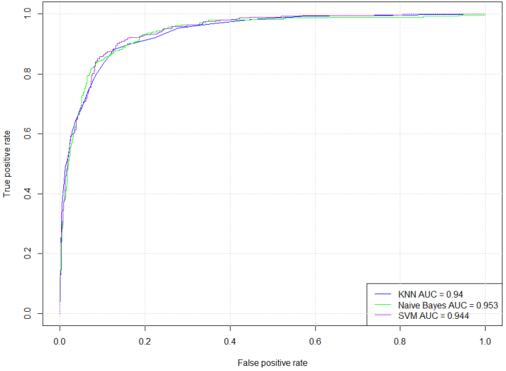
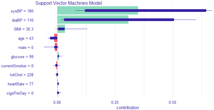
Hypertension is a major public health challenge globally, often undiagnosed until severe complications arise, highlighting the critical need for early and accurate risk prediction methods. Despite advances in machine learning (ML), many models remain black boxes, limiting clinical trust and adoption. This study addresses these gaps by evaluating and interpreting three ML classifiers—Support Vector Machine (SVM), K-Nearest Neighbors (KNN), and Naïve Bayes—for hypertension risk prediction, emphasizing both predictive performance and explainability. Using a comprehensive dataset of 4,187 participants, demographic and clinical factors, including age, gender, smoking status, blood pressure, BMI, glucose levels, and medication use, were analyzed. Descriptive statistics revealed significant differences between the at-risk and no-risk groups, particularly in terms of age, blood pressure, cholesterol levels, and diabetes prevalence. Chi-square and Welch's t-tests confirmed these distinctions (p <.001), underscoring the validity of the models' inputs. Model evaluation showed SVM as the most balanced classifier with an accuracy of 88.13% (95% CI [86.22%, 89.86%]) and substantial agreement (kappa = 0.7153). It achieved strong sensitivity (92.66%) and specificity (77.78%), alongside a favorable F1-score (0.9157), indicating robust true positive detection while minimizing false positives. KNN demonstrated high sensitivity (94.69%) but lower specificity (69.25%), with moderate overall accuracy (86.95%). Naïve Bayes, though highly sensitive (99.21%), suffered from poor specificity (34.63%), suggesting a high false-positive rate and imbalanced classification. McNemar's test indicated balanced errors only for SVM (p = 0.1036). Receiver Operating Characteristic (ROC) analysis revealed excellent discrimination for all models, with Naïve Bayes achieving an AUC of 0.953; however, this did not translate into practical reliability due to error imbalance. Explainable AI techniques, specifically SHAP values, elucidated key predictors in SVM, notably systolic and diastolic blood pressure, BMI, and heart rate, enhancing interpretability and stakeholder trust. According to the study, SVM offers the best trade-off between accuracy and interpretability for predicting hypertension risk. Integrating explainable ML models into clinical practice can improve early diagnosis, guide interventions, and inform health policies, supporting ethical, transparent, and effective AI-driven healthcare.

Published in	American Journal of Artificial Intelligence (Volume 9, Issue 2)
DOI	10.11648/j.ajai.20250902.17
Page(s)	154-166
Creative Commons	This is an Open Access article, distributed under the terms of the Creative Commons Attribution 4.0 International License (http://creativecommons.org/licenses/by/4.0/), which permits unrestricted use, distribution and reproduction in any medium or format, provided the original work is properly cited.
Copyright	Copyright © The Author(s), 2025. Published by Science Publishing Group

Keywords

Hypertension, Machine Learning, Support Vector Machine, Explainable AI, Risk Prediction, SHAP Values

1. Introduction

Machine learning is a subdivision of artificial intelligence that focuses on enabling machines and computers to mimic human learning and apply the knowledge to obtain solutions to problems

[1]

. Machine learning improves gradually through data exposure, making the machine gain more experience over time

[2]

. Machine learning is categorized into two categories, namely Supervised Machine Learning and Unsupervised Machine Learning

[3]

. Supervised Machine learning is used to learn from labelled data. The training dataset is employed to train the model to produce the correct output by attempting to map points between the input and output. Unsupervised machine learning uses unlabeled data, and the target variables are unknown

[4]

. In machine learning, there are two primary categories: classification and regression. This study will employ classification techniques and algorithms that assign predetermined output classes to input features.

Examples of classification algorithms include logistic regression, Support vector machines, Decision Trees, K-nearest neighbours (KNN), and Naïve Bayes

[5]

. The advantage of using Supervised Machine Learning is its high accuracy, as the models are trained on labeled data. The process of decision-making in supervised learning can be easily interpreted, and the pre-trained models save time and resources compared to building a model from scratch

[6]

. Machine learning also employs a single classifier, where a machine learning model is developed to address a specific challenge using a single algorithm. The algorithms used in a single classifier are Decision Trees, Support Vector Machine (SVM), K-Nearest Neighbours (KNN), Logistic Regression, and Naïve Bayes.

Hypertension, or high blood pressure, is a significant public health concern characterized by persistently elevated arterial pressure

[7]

. Its development is influenced by a complex interplay of lifestyle-related risk factors, including diet, physical inactivity, stress, and obesity

[8]

. This multifactorial nature makes hypertension a challenging condition to model statistically, as it requires careful consideration of both direct and indirect associations among variables. Applying machine learning to study hypertension enables researchers to identify significant predictors, assess risk, and develop targeted interventions for the prevention and management of hypertension. Hypertension is asymptomatic, which is why it takes time to detect, and hence it is a high-risk condition and is usually called the silent killer

[9]

. The prevalence rate is well known to be higher in developing countries, although clinical estimates indicate that approximately 10 percent of the total world population is affected

[10]

. It highlights the need for data-driven methods to identify crucial predictors and model the development and risk status associated with hypertension, particularly in populations experiencing rapid urbanization and lifestyle changes.

In their study to predict hypertension,

[11]

used logistic regression and SHAP values. The study involved 10,000 individuals and examined clinical factors, including age, BMI, Blood pressure, and lifestyle factors such as sodium intake and physical activity. A logistic model was trained to predict the presence of hypertension. The model yielded an AUC-ROC of 0.88, and SHAP values revealed that age, BMI, and sodium intake were the most significant predictors of hypertension. The study utilized data from at least 15,000 individuals, incorporating lifestyle and clinical factors. Feature importance was used to interpret the results. The model achieved an accuracy of 92%, and the importance analysis identified age, BMI, and physical inactivity as the top predictors of hypertension. The study could have utilized XAI for explainability.

In their study,

[12]

applied Neural networks and LIME to predict hypertension and interpret he results. The study used electronic health records from 20,000 patients, a neural network model was trained, and LIME was used to interpret the results. The results indicated that an AUC_ROC of 0.91 was achieved, with family history and high cholesterol being the main predictors.

[13]

predicted hypertension using gradient boosting and interpreted the results using SHAP. The study utilized a dataset of 12,000 individuals, incorporating clinical and lifestyle variables. The results indicated that an ROC accuracy of 0.89 was achieved, with age, BMI, and sodium intake being the most influential predictors.

Based on the global burden of hypertension and its clinical and lifestyle adverse outcomes, this subsection summarizes the predictive performance of three machine learning (ML) algorithms that will be used in this study: Support Vector Machine (SVM), K-Nearest Neighbours (KNN), and Naïve Bayes (NB) in the domain of health-related data classification. The models have been influential in medical research because they can process various types of data and facilitate early-stage disease detection, such as hypertension, diabetes, and cardiovascular diseases.

The other classification method commonly used is the Support Vector Machine (SVM), which is particularly effective when working with large-dimensional datasets and when the classification process involves binary classification

[14]

. Its kernel functions befit a non-linear and sophisticated relationship between disease outcomes and health indicators. The prediction of cardiovascular disease and hypertension using SVM has been effectively employed in various studies worldwide. For example, studies using Asian and European population datasets have demonstrated that SVM can achieve both high recall and high precision in predicting hypertension

[15]

. Nevertheless, SVM models usually require fine-tuning and feature scaling, which will be part of the research design in question.

K-Nearest Neighbors (KNN) is an instance learning algorithm that is based on the distance between instances and is both very simple and easy to understand

[16]

. KNN has been successfully applied in predictive models of diverse non-communicable diseases globally. Studies in Africa, South America, and the U.S. show that KNN gives satisfactory results when the dataset is balanced and has no noise. However, it is weak in handling irrelevant features and imbalanced classes

[17]

. KNN can also be used as a base comparison in the modeling of hypertension, as opposed to being the first choice, due to its high computational complexity, and the parameter k needs to be carefully selected. Naïve Bayes (NB) is a probabilistic classifier that assumes independence among the predictors. Despite this supposition, NB is competitive in accuracy, especially in health studies that comprise extensive categorical data

[18]

. It has been used not only on all continents, such as in conducting research in Europe, the Middle East, and the U.S., but also in classifying diseases like hypertension and other cardiovascular conditions.

To assess and compare the performance of the chosen machine learning models —Support Vector Machine (SVM), K-Nearest Neighbours (KNN), and Naïve Bayes (NB) —the research will utilize standard classification measures applied in medical prediction. These are the accuracy that provides the overall correctness of the model, precision that shows the true positive predictions in proportion to all positive predictions, and recall (sensitivity) as an expression of the capacity to distinguish correctly among hypertensive patients. Additionally, a harmonic average of precision and recall, defined as the F1-score, was calculated to provide an unbiased picture (in the case of non-imbalanced classes) of the models. The Receiver Operating Characteristic (ROC) curve and the Area Under the Curve (AUC), where applicable, were used to determine the diagnostic potential of the models at various classification limits. These measures will ensure an extensive and impartial assessment of the efficacy of all algorithms in predicting the development of hypertension, taking into account clinical and lifestyle data.

2. Research Materials and Methods

2.1. Research Design

This study used a dataset from Kaggle (Hypertension-risk-model-main). The primary objectives are to examine the key characteristics, such as age, systolic and diastolic blood pressure, cholesterol level, and glucose level, present within the dataset. Leveraging an existing dataset in Kaggle offers efficiency and cost-effectiveness, although the selected variables might constrain the research. Due to this, the dataset was carefully considered for quality and documentation.

2.2. Data Collection

Data collection refers to the process of gathering information for research purposes. The research study utilized secondary data, as defined by

[18, 19]

. Secondary data are data that were initially collected for another purpose and can be further analyzed to provide additional or different information, interpretations, and conclusions. Secondary data for the study were obtained and downloaded from Kaggle Hypertension-risk-model-main.

2.3. Data Analysis

2.3.1. Data Partitioning

To build machine learning models, the data was partitioned into training, testing, and validation sets, as described by

[20]

. As presented in Table 1, this study utilized 70% of the data for testing and training the k-Nearest Neighbors (KNN), Naïve Bayes, and Support Vector Machine (SVM) models. The 70/30 split provides sufficient distinct data to test the model's performance in unseen situations while also allowing for efficient training of the model

[21, 22]

. The caret package in R was used to split the data into a training and testing set. The function createDataPartition() plays a role in maintaining the distribution of the outcome variable, which is responsible for classification during data splitting

[23]

Table 1. Data Partitioning into Training and Testing for Machine Learning.

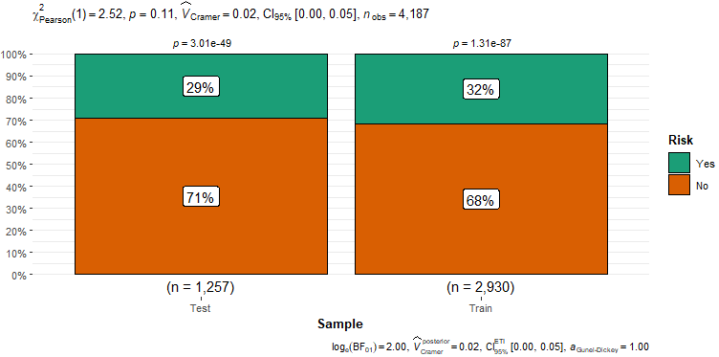
Sample	Risk		Total
Sample	No	Yes	Total
Test	890	367	1257
	70.8%	29.2%	100%
	30.8%	28.3%	30%
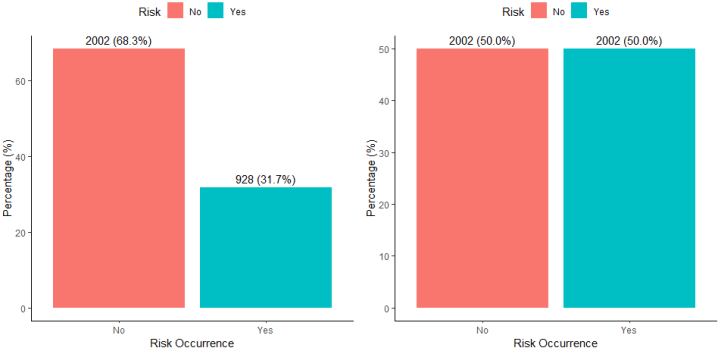
Train	2002	928	2930
	68.3%	31.7%	100%
	69.2%	71.7%	70%
Total	2892	1295	4187
	69.1%	30.9%	100%
	100%	100%	100%
χ²=2.409 · df=1 · &phi=0.025 · p=0.121

The dataset was divided into training and testing subsets to facilitate model development and evaluation. The training set comprised 2,930 observations (70% of the total), with 2,002 (68.3%) labeled as "No" risk and 928 (31.7%) as "Yes" risk. The test set included 1,257 observations (30% of the total), containing 890 (70.8%) "No" risk and 367 (29.2%) "Yes" risk cases. Overall, the full dataset consisted of 4,187 observations, with 2,892 (69.1%) "No" risk and 1,295 (30.9%) "Yes" risk cases. A chi-square test revealed no statistically significant difference in risk distribution between the training and test sets, χ²(1) = 2.409, p =.121, indicating that the partitioning preserved the proportional distribution of risk categories across the subsets.

Download: Download full-size image

Figure 1. Data Partitioning and Cases Proportional Testing.

Figure 1 above illustrates the distribution of a binary 'Risk' variable across 'Test' and 'Train' data partitions. The plot is a stacked bar chart showing the composition of each sample. The 'Test' partition contains 1,257 observations, with 71% categorized as 'No Risk' and 29% as 'Yes Risk'. The larger 'Train' partition, with 2,930 observations, shows a similar distribution of 68% 'No Risk' and 32% 'Yes Risk'. A Pearson's χ² test, with a value of χ²(1) =2.52, was conducted to compare the risk distribution between the two samples. The resulting p-value of 0.11 indicates that there is no statistically significant difference in the composition of the risk variable across the two data partitions

[24]

. This suggests that the data was successfully split into two representative and unbiased samples, suitable for tasks such as training and evaluating a machine learning model

[25]

2.3.2. Data Balancing

The bar plot depicts the percentage of "No Risk" and "Yes Risk" occurrences across two distinct datasets. The left plot presents an imbalanced distribution, where "No Risk" constitutes 68.3% (n = 2002) of the observations, while "Yes Risk" represents 31.7% (n = 928). In contrast, the right plot shows a perfectly balanced dataset, with "No Risk" and "Yes Risk" each accounting for 50% (n = 2002) of the total observations. This plot illustrates the contrast between the original, imbalanced data and a resampled, balanced version, a common practice in machine learning to mitigate model bias towards the majority class (Brownlee, 2020). During the exploratory phase, data balancing using the synthetic minority over-sampling technique (SMOTE) was considered due to the class imbalance (68.3% 'No Risk' vs. 31.7% 'Yes Risk'). The final models were trained on the balanced data and tested on the testing dataset to avoid potential bias introduced by the imbalanced nature of the clinical data.

Download: Download full-size image

Figure 2. Balanced and Imbalanced Data.

2.3.3. Machine Learning Models Development

This section provides detailed information on how each machine learning model, such as k-Nearest Neighbors (KNN), Naïve Bayes, and Support Vector Machine (SVM), will be developed. Each model is selected for its unique characteristics, including data handling, interpretability, accuracy, and computational efficiency.

I. Training K-Nearest Neighbors (KNN)

KNN is one of the models whose training phase is very explicit; the model operates by memorizing the entire training data and using it directly to make predictions

[26]

. The feature vectors and their corresponding labels are stored from the datasets. Let the training data be represented by

D = \{(x_{1}, y_{1}), (x_{2}, y_{2}), \dots, x_{n}, y_{n}\}

(1)

Where

x_{1}, y_{1} These End

Equations are labels for class classification. KNN stores the data in terms of training instances and computer distances, that is, Euclidean distances

x

and training data

xi

[27]

ⅆ (x, x_{i}) = \sqrt{\sum_{j = 1} {(x_{i} - x_{j})}^{2}}

(2)

Where

ω ⅈ = \frac{1}{ⅆ (x, x_{i})}

Applies inverse weighting to neighbors based on distance.

II. Training Naïve Bayes

The Bayes' theorem assumes that the probability of a class is known.

C

In the presence of some features.

X = x_{1} . x_{2}, \dots x_{n}

(3)

Bayes' theorem is written as

P (C| X) = \frac{P (X | C) \cdot P (C)}{P (X)}

(4)

During the training phase, the algorithm learns the prior probabilities.

P (C)

and likelihoods

P (x_{i}| C)

[28]

. For each class, the training data is used to assign each feature provided in the class. The training data is represented as:

D = \{(x_{1}, y_{1}), (x_{2}, y_{2}), \dots, (x_{n}, y_{n})\}

(5)

where

x_{i}^{'} s

Is the feature vector for

i^{th}

data and

yi .

These are the class labels. The classes are

K classes C_{1}, C_{2}, \dots, C_{k}

. The posterior probability is used for prediction, and the class with the highest posterior probability is selected for classification. The logarithmic form is as follows:

\log_{P} (Y = c| x) = \log P (Y = c) + \sum_{j = 1}^{p} logP (x_{j} | Y = c

(6)

Laplace smoothing is applied to ensure that the challenge of zero probability does not affect the model

[29]

. When a particular class lacks a feature value that does not appear in the training data, a small constant is added to the count.

α = 1

of each feature.

P (x_{i} | C_{k}) = \frac{Count of xi in class C_{k} + α}{Total count for all features in class C_{k} + α . |V|}

(7)

III. Training Support Vector Machine (SVM)

SVM is a robust and supervised learning algorithm used for classification that operates by finding an optimal hyperplane that increases the margin between different classes in feature space

[30]

. The closest points are referred to as support vectors. For a binary classification, given the dataset

= \{(x_{1}, y_{1}), (x_{2}, y_{2}), \dots, (x_{n}, y_{n})\}

. The hyperplane is defined as follows:

w^{T} x + b = 0

(8)

W

being the weight vector,

b

is the intercept, and

x

is the feature vector

[31]

. The next step is to maximize the distance between the hyperplane and the closest data points, which is expressed as

\frac{2}{‖W‖}

. The correct classification of all training points should be considered, which is why the condition below must be met, allowing at least a margin of 1.

y ⅈ c w^{T} x_{i} + b \geq 1, \forall ⅈ

(9)

The optimization problem of finding the optimal hyperplane is solved by maximizing the margin

[32]

. This is done by introducing the Lagrange multipliers, and the optimization problem is converted to,

L (w, b, α) = \frac{1}{2} {‖w‖}^{2} - \sum_{i = 1}^{n} α_{i} [y_{i} (w^{T} x_{i} + b)] - 1]

(10)

Where

αi

is the Lagrange multiplier, and

L

is maximized with respect to

α

and minimized with respect to

w and b .

Once the SVM model is trained, the decision function is evaluated:

\hat{y} = sign (\sum_{i = 1}^{N} α_{i} y_{i} K (x_{i}, x) + b)

(11)

2.3.4. Cross Validation

Model generalizability is a crucial feature in machine learning, and this study utilized 10-fold cross-validation during the model training process

[33]

. The data was partitioned into ten subsets, nine of which will be used for training and one for validation. This will ensure that there is no overfitting

[34]

2.3.5. Hyperparameter Tuning

Hyperparameter tuning is a significant step in optimizing machine learning models. Hyperparameters are set before the training process to control how the models learn

[35]

. In this study, parameter tuning was considered in all the models using grid search optimization. This process ensures the model's generalization, reliability, and accuracy, thereby reducing the risks of overfitting and underfitting.

3. Results and Discussion

3.1. Descriptive Statistics

Table 2 shows the descriptive statistics for the study variables. The total sample consisted of 4,187 participants. The mean age of participants was 49.53 years (SD = 8.56), with a median of 49, a minimum of 32, and a maximum of 70 years. Age distribution showed slight positive skewness (Skew = 0.23) and moderate negative kurtosis (Kurtosis = -0.99), indicating a fairly symmetrical distribution. Gender was coded as a binary variable (1 = Female, 2 = Male), with a mean of 1.43 (SD = 0.50), suggesting a slightly higher proportion of females. The skewness for gender was 0.28 with a negative kurtosis of -1.92, showing a moderate deviation from normality. Current smoking status, also coded as binary (1 = Non-smoker, 2 = Smoker), had a mean of 1.49 (SD = 0.50) and showed minimal skew (0.02) but strong negative kurtosis (-2.00), indicating a relatively flat distribution.

The number of cigarettes smoked per day had a highly skewed distribution (Skew = 1.25, Kurtosis = 1.04), with a mean of 9.02 (SD = 11.88) and a median of 0. This suggests that many individuals did not smoke, while a small number smoked heavily. Blood pressure medication usage (1 = not on medication, 2 = on medication) had a mean of 1.03 (SD = 0.17), with strong positive skewness (5.55) and high kurtosis (28.78), indicating that most participants were not taking medication. Similarly, diabetes status (1 = non-diabetic, 2 = Diabetic) had a mean of 1.03 (SD = 0.16), skew = 6.01, and kurtosis = 34.14, again reflecting a low prevalence of diabetes. Total cholesterol had a mean of 236.65 mg/dL (SD = 44.22), ranging from 107 to 696 mg/dL, with moderate skewness (0.88) and leptokurtic distribution (Kurtosis = 4.28). Systolic blood pressure averaged 132.29 mmHg (SD = 21.98), and diastolic pressure averaged 82.89 mmHg (SD = 11.88), both showing moderate right skew and kurtosis. BMI had a mean of 25.80 (SD = 4.07), showing mild positive skewness (0.98) and moderate kurtosis (2.69). The heart rate had a mean of 75.88 bpm (SD = 12.05), and the glucose level had a mean of 81.96 mg/dL (SD = 22.90), with glucose exhibiting high positive skew (6.53) and extreme kurtosis (64.78), indicating the presence of outliers with abnormally high glucose levels. Lastly, the hypertension risk, coded as binary (1 = no risk, 2 = at risk), had a mean of 1.31 (SD = 0.46), skew = 0.82, and kurtosis = -1.32, indicating a slightly right-skewed distribution concentrated toward the "no risk" group.

Table 2. Descriptive Statistics.

Variables	N	Mean	SD	Median	Skew	Kurtosis	SE
Gender	4187	1.4311	0.4953	1.0000	0.2782	-1.9231	0.0077
Age	4187	49.5307	8.5559	49.0000	0.2333	-0.9867	0.1322
Current Smoker	4187	1.4949	0.5000	1.0000	0.0205	-2.0001	0.0077
Cigarettes Smoked Per Day	4187	9.0165	11.8784	0.0000	1.2471	1.0358	0.1836
Blood Pressure Medications	4187	1.0296	0.1695	1.0000	5.5475	28.7815	0.0026
diabetes*	4187	1.0256	0.1578	1.0000	6.0109	34.1393	0.0024
Total Cholesterol	4187	236.6528	44.2228	234.0000	0.8794	4.2823	0.6834
Systolic Blood Pressure	4187	132.2917	21.9829	128.0000	1.1454	2.1766	0.3397
Diastolic Blood Pressure	4187	82.8911	11.8785	82.0000	0.6969	1.2258	0.1836
BMI	4187	25.8035	4.0672	25.4200	0.9794	2.6944	0.0629
Heart Rate	4187	75.8767	12.0535	75.0000	0.6471	0.9030	0.1863
Glucose Level	4187	81.9584	22.9038	80.0000	6.5269	64.7770	0.3540
Hypertension Risk	4187	1.3093	0.4623	1.0000	0.8249	-1.3198	0.0071

3.2. Chi-Square Tests and Welch Two-Sample T-test

Table 3 presents a comparison of demographic and clinical characteristics between individuals classified as at risk and those not at risk, based on a total sample of 4,187 participants. Gender distribution did not significantly differ between the groups, χ² (1, N = 4,187) = 0.276, p =.600, with females representing 57% of the overall sample, and nearly identical proportions in the no-risk (57%, 95% CI [55%, 59%]) and at-risk groups (56%, 95% CI [54%, 59%]). However, a significant difference was observed in age, with the at-risk group being older (M = 53.43, SD = 8.13, 95% CI [53, 54]) than the no-risk group (M = 47.79, SD = 8.16, 95% CI [47, 48]), t(2221.7) = -20.67, p <.001. Smoking status also showed statistically significant differences, χ² (1, N = 4,187) = 55.82, p <.001, where 53% (95% CI [51%, 55%]) of individuals in the no-risk group were current smokers compared to only 42% (95% CI [39%, 45%]) in the at-risk group. While individuals in the no-risk group smoked more cigarettes per day on average (M = 9.52, SD = 11.78, 95% CI [9.1, 10]) than those at risk (M = 7.88, SD = 12.03, 95% CI [7.2, 8.5]), this difference was also statistically significant, t(4134.2) = 3.47, p <.001.

Other notable differences were observed in clinical characteristics. Individuals in the at-risk group were significantly more likely to be on blood pressure medication (9.6%, 95% CI [8.1%, 11%]) compared to none in the no-risk group (0%, 95% CI [0.00%, 0.17%]), χ² (1, N = 4,187) = 291.47, p <.001. Diabetes prevalence was also higher among the at-risk group (4.4%, 95% CI [3.4%, 5.7%]) than the no-risk group (1.7%, 95% CI [1.3%, 2.3%]), with this difference being statistically significant, χ² (1, N = 4,187) = 22.94, p <.001. Continuous clinical measures further showed significant group differences. Total cholesterol was higher among those at risk (M = 247.25, SD = 47.38, 95% CI [245, 250]) than those not at risk (M = 231.91, SD = 41.88, 95% CI [230, 233]), t(2095.4) = -11.60, p <.001. Similarly, systolic blood pressure was significantly elevated in the at-risk group (M = 155.14, SD = 20.75, 95% CI [154, 156]) compared to the no-risk group (M = 122.06, SD = 12.97, 95% CI [122, 123]), t(1754.6) = -51.26, p <.001. Diastolic blood pressure followed the same pattern (at-risk: M = 93.85, SD = 11.28, 95% CI [93, 94]; no-risk: M = 77.99, SD = 8.34, 95% CI [78, 78]), t (1517.3) = -42.96, p <.001. Other significant differences were observed in body mass index (BMI), heart rate, and glucose level. At-risk individuals had higher BMIs (M = 27.64 vs. 24.98), heart rates (M = 78.52 vs. 74.69), and glucose levels (M = 84.78 vs. 80.69), with all comparisons yielding p <.001 and non-overlapping confidence intervals, confirming statistically and clinically meaningful group distinctions.

Table 3. Chi-Square Test and Welch Two-Sample Test.

Characteristic	N	Overall	No	95% CI	Yes	95% CI	p-value²
Characteristic	N	N = 4,187¹	N = 2,892¹	95% CI	N = 1,295¹	95% CI	p-value²
male	4,187						0.6
Female		2,382 (57%)	1,652 (57%)	55%, 59%	730 (56%)	54%, 59%
Male		1,805 (43%)	1,240 (43%)	41%, 45%	565 (44%)	41%, 46%
age	4,187	49.53 (8.56)	47.79 (8.16)	47, 48	53.43 (8.13)	53, 54	<0.001
Current Smoker	4,187						<0.001
Not-Current-Smoker		2,115 (51%)	1,363 (47%)	45%, 49%	752 (58%)	55%, 61%
Current-Smoker		2,072 (49%)	1,529 (53%)	51%, 55%	543 (42%)	39%, 45%
Cigarettes Smoked Per Day	4,187	9.02 (11.88)	9.52 (11.78)	9.1, 10	7.88 (12.03)	7.2, 8.5	<0.001
Blood Pressure Medications	4,187						<0.001
Not on BP Medication		4,063 (97%)	2,892 (100%)	100%, 100%	1,171 (90%)	89%, 92%
On BP Medication		124 (3.0%)	0 (0%)	0.00%, 0.17%	124 (9.6%)	8.1%, 11%
diabetes	4,187						<0.001
Not Diabetic		4,080 (97%)	2,842 (98%)	98%, 99%	1,238 (96%)	94%, 97%
Diabetic		107 (2.6%)	50 (1.7%)	1.3%, 2.3%	57 (4.4%)	3.4%, 5.7%
Total Cholesterols	4,187	236.65 (44.22)	231.91 (41.88)	230, 233	247.25 (47.38)	245, 250	<0.001
Systolic Blood Pressure	4,187	132.29 (21.98)	122.06 (12.97)	122, 123	155.14 (20.75)	154, 156	<0.001
Diastolic Blood Pressure	4,187	82.89 (11.88)	77.99 (8.34)	78, 78	93.85 (11.28)	93, 94	<0.001
BMI	4,187	25.80 (4.07)	24.98 (3.52)	25, 25	27.64 (4.57)	27, 28	<0.001
Heart Rate	4,187	75.88 (12.05)	74.69 (11.53)	74, 75	78.52 (12.77)	78, 79	<0.001
Glucose Level	4,187	81.96 (22.90)	80.69 (19.91)	80, 81	84.78 (28.27)	83, 86	<0.001

Abbreviation: CI = Confidence Interval

¹ n (%); Mean (SD)

² Pearson's Chi-squared tests; Welch Two Sample t-test

3.3. Machine Learning Model Summary

Table 4 presents the evaluation metrics for the three machine learning models, focusing on diagnostic accuracy, 95% confidence intervals (CI), Cohen's kappa, and McNemar's test. The models were trained and tested with "Yes" as the positive class, representing individuals who have been diagnosed with hypertension. Among the models, the Support Vector Machine (SVM) demonstrated the best overall performance, achieving an accuracy of 88.13%, with a 95% CI of (0.8622, 0.8986) and a kappa value of 0.7153, reflecting substantial agreement between predicted and actual classifications. The non-significant McNemar's test p-value of 0.1036 suggests balanced error types, an important quality for clinical decision support systems. The K-Nearest Neighbors (KNN) model followed closely with 86.95% accuracy and a kappa of 0.6747, indicating moderate agreement. However, the highly significant McNemar's p-value (3.58 × 10^-8) suggests the model may be skewed in its prediction errors, potentially overpredicting one class, which could compromise sensitivity or specificity in practice. The Naïve Bayes model yielded the lowest accuracy (79.56%) and a kappa of 0.4120, indicating weak agreement beyond chance. McNemar's p-value (< 2.2 × 10^-16) is extremely significant, further suggesting a strongly unbalanced classification error pattern. Although computationally efficient, its diagnostic reliability is limited in this context. From the results, the SVM model emerges as the most balanced and reliable classifier for predicting hypertension risk among the models evaluated, combining high accuracy with a statistically sound error distribution.

Table 4. Machine Learning Model Summary Report.

Model	Accuracy	95% CI	Kappa	McNemar's Test p-value	Positive Class
KNN	0.8695	(0.8497, 0.8875)	0.6747	3.58 × 10^-8	Yes
Naïve Bayes	0.7956	(0.7724, 0.8174)	0.4120	< 2.2 × 10^-16	Yes
SVM	0.8813	(0.8622, 0.8986)	0.7153	0.1036	Yes

3.4. Machine Learning Model Performance

Table 5 presents the evaluation metrics, indicating that the Support Vector Machine (SVM) model outperformed the others in predicting hypertension risk. It demonstrated a strong balance between sensitivity (0.9266) and specificity (0.7778), indicating that it effectively identifies both at-risk and non-risk individuals. The model achieved a precision of 0.9051 and an F1-score of 0.9157, reflecting high accuracy in classifying true positive cases while minimizing false positives. Its balanced accuracy of 0.8522 and Kappa score of 0.7153 further highlight its reliability and substantial agreement beyond chance.

Although the Naïve Bayes model achieved the highest sensitivity (0.9921), its specificity was considerably lower (0.3463), suggesting a high false-positive rate. The K-Nearest Neighbors model demonstrated good sensitivity (0.9469) and acceptable precision, but had a lower specificity (0.6925) compared to the SVM. Overall, the SVM provided the most consistent and balanced performance, making it the most suitable model for predicting hypertension risk in this study.

Table 5. Machine Learning Model Performance Metrics.

Model	Sensitivity	Specificity	Precision	F1_Score	Recall	NPV	PPV	Balanced Accuracy	Kappa
K-NN	0.9469	0.6925	0.8757	0.9099	0.9469	0.8508	0.8757	0.8197	0.6747
Naïve Bayes	0.9921	0.3463	0.7763	0.8710	0.9921	0.9504	0.7763	0.6692	0.4120
Support Vector Machines	0.9266	0.7778	0.9051	0.9157	0.9266	0.8224	0.9051	0.8522	0.7153

3.5. Receiver Operating Characteristic Curve and AUC

Figure 3 presents the Receiver Operating Characteristic (ROC) curves for three machine learning models: K-Nearest Neighbors (KNN), Naïve Bayes, and Support Vector Machine (SVM). Each curve illustrates the trade-off between the True Positive Rate (Sensitivity) and the False Positive Rate (1 - Specificity) across different threshold values. The Area Under the Curve (AUC), shown in the legend, provides a quantitative measure of each model's overall classification performance. The results show that the Naïve Bayes model achieved an AUC of 0.953, indicating a near perfect classification capability. This means the model was able to perfectly distinguish between individuals at risk of hypertension and those not at risk. Such a performance reflects a highly effective understanding of the underlying patterns in the data.

In contrast, both the KNN and SVM models recorded AUC scores of 0.9, which still represent strong performance but fall slightly short of perfection. Their ROC curves lie just below that of Naïve Bayes, particularly in the mid-range of false positive rates, suggesting relatively lower sensitivity-specificity trade-offs. Overall, the Naïve Bayes model proves to be the most effective tool for predicting hypertension risk based on the clinical and lifestyle features evaluated in this study.

Download: Download full-size image

Figure 3. Receiver Operating Characteristic Curve and Area Under the Curve.

3.6. Explainable Artificial Intelligence (XAI)

To enhance the trust, transparency, and usability of machine learning models in high-stakes domains such as health diagnostics or financial risk assessment, Explainable Artificial Intelligence (XAI) plays a vital role. XAI refers to a set of techniques and tools that make the decisions and internal logic of machine learning models interpretable to human users. While complex models, such as Support Vector Machines, often offer superior predictive performance, they are typically considered "black boxes" due to their lack of interpretability.

In this study, incorporating XAI methods such as SHAP (SHapley Additive exPlanations) or LIME (Local Interpretable Model-Agnostic Explanations) would help users understand the contribution of each input variable to the model's prediction. This is especially important for building stakeholder trust, facilitating policy uptake, and ensuring that the model's decisions can be scrutinized for fairness and bias. Future work should prioritize the integration of such techniques to support the ethical and transparent deployment of these systems.

3.6.1. Shapley Additive Explanations

Download: Download full-size image

Figure 4. SHapley Additive Explanations for Support Vector Machines.

Figure 4 displays the feature contributions to a Support Vector Machine model's prediction. The two most impactful features are systolic blood pressure (sysBP) at 180 mmHg and diastolic blood pressure (diaBP) at 110 mmHg. Both have significant positive contributions, with sysBP being the largest. Other features, such as BMI (30.3) and heart rate (77), also have positive but smaller contributions. Conversely, age (43) and being female (male=0) show minor negative contributions, suggesting they slightly decrease the model's output. The remaining features have minimal impact.

3.6.2. Model Breakdown

Download: Download full-size image

Figure 5. Support Vector Machines Model Breakdown.

Figure 5 shows the "Breakdown profile" plot, which visualizes the contribution of various factors to a Support Vector Machine model's prediction. The final prediction is 0.99. The intercept contributes 0.313. A systolic blood pressure (sysBP) of 180 is the most significant positive contributor, adding 0.647 to the model. Other factors, such as a diastolic blood pressure (diaBP) of 110, a BMI of 30.3, and a heart rate of 77, also contribute positively, albeit to a lesser extent. Gender (male=0), smoking status (currentSmoker=0), and other combined factors have minor negative contributions.

4. Conclusions and Recommendations

This study aimed to develop and evaluate machine learning models for predicting binary risk status ("Yes" or "No") using supervised classification techniques. The primary objective was to identify the most effective model among k-Nearest Neighbors (KNN), Naïve Bayes, and Support Vector Machines (SVM), based on diagnostic performance metrics including accuracy, sensitivity, specificity, precision, Cohen's kappa, and McNemar's test. Among the evaluated models, the Support Vector Machine (SVM) emerged as the most balanced and robust performer, achieving an accuracy of 88.13%, a kappa of 0.7153, a sensitivity of 92.66%, and a specificity of 77.78%. The non-significant McNemar's test p-value (0.1036) indicates consistent classification without statistically significant error imbalance. KNN followed closely with 86.95% accuracy, high sensitivity (94.69%), but comparatively lower specificity (69.25%), suggesting a tendency to overpredict the positive class. Naïve Bayes, while delivering the highest sensitivity (99.21%), exhibited poor specificity (34.63%), resulting in a model that is heavily imbalanced and favors false positives. Based on these findings, SVM stands out as the most reliable model for risk prediction in this context. Practitioners and policymakers can adopt this model in decision-support systems for public health screening, financial risk assessment, or educational interventions targeting specific populations. Its balance between sensitivity and specificity makes it especially suitable for high-stakes applications, where minimizing both false negatives and false positives is critical. Policy frameworks should advocate for the integration of machine learning into risk management practices and invest in capacity-building initiatives to improve data literacy and model transparency. Future studies should emphasize explainable AI techniques, external validation on diverse populations, and evaluation in real-world environments to enhance the utility and trustworthiness of predictive models.

Abbreviations

ML	Machine Learning
KNN	K-Nearest Neighbors
SVM	Support Vector Machines
NB	Naïve Bayes
ROC	Receiver Operating Characteristic
AUC	Area Under the Curve
NPV	Negative Predictive Value
PPV	Positive Predictive Value
F1	F1 Score (Harmonic Mean of Precision and Recall)
Sens	Sensitivity (True Positive Rate)
Spec	Specificity (True Negative Rate)

Acknowledgments

First and foremost, we give all glory and honor to the Almighty God, whose grace, wisdom, and strength have guided me throughout this academic journey. Special thanks to Chuka University, Department of Physical Science, and the Centre for Data Analytics and Modelling (CDAM), whose academic environment and support provided the foundation needed to conduct and complete this study. This work is a collective achievement, made possible by the many people who walked with me along the way. To all who contributed in one way or another, we would like to extend our sincere gratitude.

Author Contributions

Elizabeth Wahito Waburi: Conceptualization, Data curation, Formal Analysis, Methodology, writing, original draft, Writing - review & editing

Dennis K. Muriithi: Conceptualization, Data curation, Formal Analysis, Methodology, writing original draft, Writing, review & editing

Sunday Mukhwana: Conceptualization, Data curation, Formal Analysis, Methodology, writing original draft, Writing review & editing

Funding

The research received no external funding.

Data Availability Statement

The data is available from the corresponding author upon reasonable request.

Conflicts of Interest

The authors declare no conflicts of interest.

References

[1]	Bekbolatova, M., Mayer, J., Ong, C. W., & Toma, M. (2024). Transformative Potential of AI in Healthcare: Definitions, Applications, and Navigating the Ethical Landscape and Public Perspectives. Healthcare, 12(2), 125-125. https://doi.org/10.3390/healthcare12020125
[2]	Muriithi, D. K., Lumumba, V. W., Awe, O. O., & Muriithi, D. M. (2025). An Explainable Artificial Intelligence Models for Predicting Malaria Risk in Kenya. European Journal of Artificial Intelligence and Machine Learning, 4(1), 1-8. https://doi.org/10.24018/ejai.2025.4.1.47
[3]	Pugliese, R., Regondi, S., & Marini, R. (2021). Machine learning-based approach: Global trends, research directions, and regulatory standpoints. Data Science and Management, 4, 19-29. Science direct. https://doi.org/10.1016/j.dsm.2021.12.002
[4]	Yazici, İ., Shayea, I., & Din, J. (2023). A survey of applications of artificial intelligence and machine learning in future mobile networks-enabled systems. Engineering Science and Technology, an International Journal, 44, 101455. https://doi.org/10.1016/j.jestch.2023.101455
[5]	Alnuaimi, A. F. A. H., & Albaldawi, T. H. K. (2024). An overview of machine learning classification techniques. Bio Web of Conferences/BIO Web of Conferences, 97(4), 00133-00133. https://doi.org/10.1051/bioconf/20249700133
[6]	Han, X., Zhang, Z., Ding, N., Gu, Y., Liu, X., Huo, Y., Qiu, J., Zhang, L., Han, W., Huang, M., Jin, Q., Lan, Y., Liu, Y., Liu, Z., Lu, Z., Qiu, X., Song, R., Tang, J., Wen, J.-R., & Yuan, J. (2021). Pre-Trained Models: Past, Present and Future. AI Open, 2. https://doi.org/10.1016/j.aiopen.2021.08.002
[7]	Oparil, S., Acelajado, M. C., Bakris, G. L., Berlowitz, D. R., Cífková, R., Dominiczak, A. F., Grassi, G., Jordan, J., Poulter, N. R., Rodgers, A., & Whelton, P. K. (2019). Hypertension. Nature Reviews Disease Primers, 4(4), 1-48. https://doi.org/10.1038/nrdp.2018.14
[8]	Charchar, F. J., Prestes, P. R., Mills, C., Ching, S. M., Neupane, D., Marques, F. Z., Sharman, J. E., Vogt, L., Burrell, L. M., Korostovtseva, L., Zec, M., Patil, M., Schultz, M. G., Wallen, M. P., Renna, N. F., Islam, S. M. S., Hiremath, S., Gyeltshen, T., Chia, Y.-C., & Gupta, A. (2023). Lifestyle management of hypertension: International Society of Hypertension position paper endorsed by the World Hypertension League and European Society of Hypertension. Journal of Hypertension, 42(1), 23-49. https://doi.org/10.1097/HJH.0000000000003563
[9]	Iqbal, A. M., & Jamal, S. F. (2023, July 20). Essential Hypertension. Nih.gov; StatPearls Publishing. https://www.ncbi.nlm.nih.gov/books/NBK539859/
[10]	Islam, M. N., Alam, Md. J., Maniruzzaman, Md., Ahmed, N. A. M. F., Ali, M., Md. Jahanur Rahman, & Dulal Chandra Roy. (2023). Predicting the risk of hypertension using machine learning algorithms: A cross sectional study in Ethiopia. PLOS ONE, 18(8), e0289613-e0289613. https://doi.org/10.1371/journal.pone.0289613
[11]	Patel, R. (2021). Predictive analytics in business analytics: Decision tree. Advances in Decision Sciences, 26(1), 1-30. https://doi.org/10.47654/v26y2022i1p1-30
[12]	Lee, H. (2022). Gradient boosting for hypertension prediction: SHAP-based interpretability analysis. BMC Medical Informatics and Decision Making, 22(1).
[13]	Montagna, S., Pengo, M. F., Ferretti, S., Borghi, C., Ferri, C., Grassi, G., Muiesan, M. L., & Parati, G. (2022). Machine Learning in Hypertension Detection: A Study on World Hypertension Day Data. Journal of Medical Systems, 47(1). https://doi.org/10.1007/s10916-022-01900-5
[14]	Shi, Y., Yang, K., Yang, Z., & Zhou, Y. (2021). Primer on artificial intelligence. Elsevier EBooks, 7-36. https://doi.org/10.1016/b978-0-12-823817-2.00011-5
[15]	Sanchez, T. R., Inostroza-Nieves, Y., Hemal, K., & Chen, W. (2023). Cross-sectional study. Translational Surgery, 219-222. https://doi.org/10.1016/b978-0-323-90300-4.00030-6
[16]	Sileyew, K. J. (2019). Research Design and Methodology. Text Mining - Analysis, Programming and Application, 7(1), 1-12. Intechopen. https://doi.org/10.5772/intechopen.85731
[17]	Xiong, L. & Yao, Y. (2021). Study on an adaptive thermal comfort model with K-nearest-neighbors (Knn) algorithm. Building and Environment, 202, 108026. https://doi.org/10.1016/j.buildenv.2021.108026
[18]	Ebid, A. E., Deifalla, A. F., & Onyelowe, K. C. (2024). Data Utilization and Partitioning for Machine Learning Applications in Civil Engineering. Sustainable Civil Infrastructures, 87-100. https://doi.org/10.1007/978-3-031-70992-0_8
[19]	Mienye, I. D., & Jere, N. (2024). A Survey of Decision Trees: Concepts, Algorithms, and Applications. IEEE Access, 4, 1-1. https://doi.org/10.1109/access.2024.3416838
[20]	Muriithi, D., Lumumba, V., & Okongo, M. (2024). A Machine Learning-Based Prediction of Malaria Occurrence in Kenya. American Journal of Theoretical and Applied Statistics, 13(4), 65-72. https://doi.org/10.11648/j.ajtas.20241304.11
[21]	Guy, R. T., Santago, P., & Langefeld, C. D. (2012). Bootstrap aggregating of alternating decision trees to detect sets of SNPs that associate with disease. Genetic Epidemiology, 36(2), 99-106. https://doi.org/10.1002/gepi.21608
[22]	Parimbelli, E., Buonocore, T. M., Nicora, G., Michalowski, W., Wilk, S., & Bellazzi, R. (2023). Why did AI get this one wrong? — Tree-based explanations of machine learning model predictions. Artificial Intelligence in Medicine, 135, 102471. https://doi.org/10.1016/j.artmed.2022.102471
[23]	Castillo-Botón, C., Casillas-Pérez, D., Casanova-Mateo, C., Ghimire, S., Cerro-Prada, E., Gutierrez, P. A., Deo, R. C., & Salcedo-Sanz, S. (2022). Machine learning regression and classification methods for fog events prediction. Atmospheric Research, 272, 106157. https://doi.org/10.1016/j.atmosres.2022.106157
[24]	Halder, R. K., Uddin, M. N., Uddin, Md. A., Aryal, S., & Khraisat, A. (2024). Enhancing K-nearest neighbor algorithm: a comprehensive review and performance analysis of modifications. Journal of Big Data, 11(1). https://doi.org/10.1186/s40537-024-00973-y
[25]	Lumumba, V., Kiprotich, D., Mpaine, M., Makena, N., & Kavita, M. (2024). Comparative Analysis of Cross-Validation Techniques: LOOCV, K-folds Cross-Validation, and Repeated K-folds Cross-Validation in Machine Learning Models. American Journal of Theoretical and Applied Statistics, 13(5), 127-137. https://doi.org/10.11648/j.ajtas.20241305.13
[26]	Lumumba, V. W., Wanjuki, T. M., & Njoroge, E. W. (2025). Evaluating the Performance of Ensemble and Single Classifiers with Explainable Artificial Intelligence (XAI) on Hypertension Risk Prediction. Computational Intelligence and Machine Learning, 6(1). https://doi.org/10.36647/ciml/06.01.a004
[27]	Sakai, T. (2025). The probability smoothing problem: Characterizations of the laplace method. Mathematical Social Sciences, 102409-102409. https://doi.org/10.1016/j.mathsocsci.2025.102409
[28]	Li, H., Jiang, L., Ganaa, E. D., Li, P., & Shen, X.-J. (2025). Robust feature enhanced deep kernel support vector machine via low rank representation and clustering. Expert Systems with Applications, 271, 126612. https://doi.org/10.1016/j.eswa.2025.126612
[29]	Muriithi, D, K., L. (2021). A machine learning approach for the prediction of surgical outcomes. American Journal of Theoretical and Applied Statistics, 9(5), 57-64.
[30]	Witten, I. H., Frank, E., Hall, M. A., & Pal, C. J. (2016). Extending instance-based and linear models. Elsevier EBooks, 243-284. https://doi.org/10.1016/b978-0-12-804291-5.00007-6
[31]	Berggren, M., Kaati, L., Pelzer, B., Stiff, H., Lundmark, L., & Akrami, N. (2024). The generalizability of machine learning models of personality across two text domains. Personality and Individual Differences, 217, 112465. https://doi.org/10.1016/j.paid.2023.112465
[32]	Zhang, M. (2021). Predicting hypertension using logistic regression and SHAP values: A clinical and lifestyle factor analysis. Journal of Medical Informatics, 45(3), 123-134.
[33]	Ilemobayo, J. A., Durodola, O., Alade, O., Awotunde, O. J., Olanrewaju, A. T., Falana, O., Ogungbire, A., Osinuga, A., Ogunbiyi, D., Ifeanyi, A., Odezuligbo, I. E., & Edu, O. E. (2024). Hyperparameter Tuning in Machine Learning: A Comprehensive Review. Journal of Engineering Research and Reports, 26(6), 388-395. https://doi.org/10.9734/jerr/2024/v26i61188
[34]	Qiu, J. (2024). An Analysis of Model Evaluation with Cross-Validation: Techniques, Applications, and Recent Advances. Advances in Economics Management and Political Sciences, 99(1), 69-72. https://doi.org/10.54254/2754-1169/99/2024OX0213
[35]	Santos, M. S., Soares, J. P., Abreu, P. H., Araujo, H., & Santos, J. (2018). Cross-Validation for Imbalanced Datasets: Avoiding Overoptimistic and Overfitting Approaches [Research Frontier]. IEEE Computational Intelligence Magazine, 13(4), 59-76. https://doi.org/10.1109/mci.2018.2866730

Cite This Article

Plain Text BibTeX RIS

APA Style

Waburi, E. W., Muriithi, D. K., Sundays, E. M. (2025). Integrating Explainable Machine Learning Models for Early Detection of Hypertension: A Transparent Approach to AI-Driven Healthcare. American Journal of Artificial Intelligence, 9(2), 154-166. https://doi.org/10.11648/j.ajai.20250902.17

Copy | Download

ACS Style

Waburi, E. W.; Muriithi, D. K.; Sundays, E. M. Integrating Explainable Machine Learning Models for Early Detection of Hypertension: A Transparent Approach to AI-Driven Healthcare. Am. J. Artif. Intell. 2025, 9(2), 154-166. doi: 10.11648/j.ajai.20250902.17

Copy | Download

AMA Style

Waburi EW, Muriithi DK, Sundays EM. Integrating Explainable Machine Learning Models for Early Detection of Hypertension: A Transparent Approach to AI-Driven Healthcare. Am J Artif Intell. 2025;9(2):154-166. doi: 10.11648/j.ajai.20250902.17

Copy | Download

@article{10.11648/j.ajai.20250902.17,
  author = {Elizabeth Wahito Waburi and Dennis Kariuki Muriithi and Eugine Mukhwana Sundays},
  title = {Integrating Explainable Machine Learning Models for Early Detection of Hypertension: A Transparent Approach to AI-Driven Healthcare
},
  journal = {American Journal of Artificial Intelligence},
  volume = {9},
  number = {2},
  pages = {154-166},
  doi = {10.11648/j.ajai.20250902.17},
  url = {https://doi.org/10.11648/j.ajai.20250902.17},
  eprint = {https://article.sciencepublishinggroup.com/pdf/10.11648.j.ajai.20250902.17},
  abstract = {Hypertension is a major public health challenge globally, often undiagnosed until severe complications arise, highlighting the critical need for early and accurate risk prediction methods. Despite advances in machine learning (ML), many models remain black boxes, limiting clinical trust and adoption. This study addresses these gaps by evaluating and interpreting three ML classifiers—Support Vector Machine (SVM), K-Nearest Neighbors (KNN), and Naïve Bayes—for hypertension risk prediction, emphasizing both predictive performance and explainability. Using a comprehensive dataset of 4,187 participants, demographic and clinical factors, including age, gender, smoking status, blood pressure, BMI, glucose levels, and medication use, were analyzed. Descriptive statistics revealed significant differences between the at-risk and no-risk groups, particularly in terms of age, blood pressure, cholesterol levels, and diabetes prevalence. Chi-square and Welch's t-tests confirmed these distinctions (p <.001), underscoring the validity of the models' inputs. Model evaluation showed SVM as the most balanced classifier with an accuracy of 88.13% (95% CI [86.22%, 89.86%]) and substantial agreement (kappa = 0.7153). It achieved strong sensitivity (92.66%) and specificity (77.78%), alongside a favorable F1-score (0.9157), indicating robust true positive detection while minimizing false positives. KNN demonstrated high sensitivity (94.69%) but lower specificity (69.25%), with moderate overall accuracy (86.95%). Naïve Bayes, though highly sensitive (99.21%), suffered from poor specificity (34.63%), suggesting a high false-positive rate and imbalanced classification. McNemar's test indicated balanced errors only for SVM (p = 0.1036). Receiver Operating Characteristic (ROC) analysis revealed excellent discrimination for all models, with Naïve Bayes achieving an AUC of 0.953; however, this did not translate into practical reliability due to error imbalance. Explainable AI techniques, specifically SHAP values, elucidated key predictors in SVM, notably systolic and diastolic blood pressure, BMI, and heart rate, enhancing interpretability and stakeholder trust. According to the study, SVM offers the best trade-off between accuracy and interpretability for predicting hypertension risk. Integrating explainable ML models into clinical practice can improve early diagnosis, guide interventions, and inform health policies, supporting ethical, transparent, and effective AI-driven healthcare.
},
 year = {2025}
}

Copy | Download

TY  - JOUR
T1  - Integrating Explainable Machine Learning Models for Early Detection of Hypertension: A Transparent Approach to AI-Driven Healthcare

AU  - Elizabeth Wahito Waburi
AU  - Dennis Kariuki Muriithi
AU  - Eugine Mukhwana Sundays
Y1  - 2025/09/23
PY  - 2025
N1  - https://doi.org/10.11648/j.ajai.20250902.17
DO  - 10.11648/j.ajai.20250902.17
T2  - American Journal of Artificial Intelligence
JF  - American Journal of Artificial Intelligence
JO  - American Journal of Artificial Intelligence
SP  - 154
EP  - 166
PB  - Science Publishing Group
SN  - 2639-9733
UR  - https://doi.org/10.11648/j.ajai.20250902.17
AB  - Hypertension is a major public health challenge globally, often undiagnosed until severe complications arise, highlighting the critical need for early and accurate risk prediction methods. Despite advances in machine learning (ML), many models remain black boxes, limiting clinical trust and adoption. This study addresses these gaps by evaluating and interpreting three ML classifiers—Support Vector Machine (SVM), K-Nearest Neighbors (KNN), and Naïve Bayes—for hypertension risk prediction, emphasizing both predictive performance and explainability. Using a comprehensive dataset of 4,187 participants, demographic and clinical factors, including age, gender, smoking status, blood pressure, BMI, glucose levels, and medication use, were analyzed. Descriptive statistics revealed significant differences between the at-risk and no-risk groups, particularly in terms of age, blood pressure, cholesterol levels, and diabetes prevalence. Chi-square and Welch's t-tests confirmed these distinctions (p <.001), underscoring the validity of the models' inputs. Model evaluation showed SVM as the most balanced classifier with an accuracy of 88.13% (95% CI [86.22%, 89.86%]) and substantial agreement (kappa = 0.7153). It achieved strong sensitivity (92.66%) and specificity (77.78%), alongside a favorable F1-score (0.9157), indicating robust true positive detection while minimizing false positives. KNN demonstrated high sensitivity (94.69%) but lower specificity (69.25%), with moderate overall accuracy (86.95%). Naïve Bayes, though highly sensitive (99.21%), suffered from poor specificity (34.63%), suggesting a high false-positive rate and imbalanced classification. McNemar's test indicated balanced errors only for SVM (p = 0.1036). Receiver Operating Characteristic (ROC) analysis revealed excellent discrimination for all models, with Naïve Bayes achieving an AUC of 0.953; however, this did not translate into practical reliability due to error imbalance. Explainable AI techniques, specifically SHAP values, elucidated key predictors in SVM, notably systolic and diastolic blood pressure, BMI, and heart rate, enhancing interpretability and stakeholder trust. According to the study, SVM offers the best trade-off between accuracy and interpretability for predicting hypertension risk. Integrating explainable ML models into clinical practice can improve early diagnosis, guide interventions, and inform health policies, supporting ethical, transparent, and effective AI-driven healthcare.

VL  - 9
IS  - 2
ER  -

Copy | Download

Author Information

Elizabeth Wahito Waburi

Department of Physical Sciences, Chuka University, Chuka, Kenya

Contact Email

http://orcid.org/0009-0002-3638-3499
Dennis Kariuki Muriithi

Department of Physical Sciences, Chuka University, Chuka, Kenya

Contact Email

http://orcid.org/0000-0002-3210-0925
Eugine Mukhwana Sundays

Department of Nursing, Chuka University, Chuka, Kenya

Contact Email

http://orcid.org/0000-0002-2281-9661

Download PDF

Submit an Article

Plain Text BibTeX RIS

APA Style

Waburi, E. W., Muriithi, D. K., Sundays, E. M. (2025). Integrating Explainable Machine Learning Models for Early Detection of Hypertension: A Transparent Approach to AI-Driven Healthcare. American Journal of Artificial Intelligence, 9(2), 154-166. https://doi.org/10.11648/j.ajai.20250902.17

Copy | Download

ACS Style

Waburi, E. W.; Muriithi, D. K.; Sundays, E. M. Integrating Explainable Machine Learning Models for Early Detection of Hypertension: A Transparent Approach to AI-Driven Healthcare. Am. J. Artif. Intell. 2025, 9(2), 154-166. doi: 10.11648/j.ajai.20250902.17

Copy | Download

AMA Style

Waburi EW, Muriithi DK, Sundays EM. Integrating Explainable Machine Learning Models for Early Detection of Hypertension: A Transparent Approach to AI-Driven Healthcare. Am J Artif Intell. 2025;9(2):154-166. doi: 10.11648/j.ajai.20250902.17

Copy | Download

@article{10.11648/j.ajai.20250902.17,
  author = {Elizabeth Wahito Waburi and Dennis Kariuki Muriithi and Eugine Mukhwana Sundays},
  title = {Integrating Explainable Machine Learning Models for Early Detection of Hypertension: A Transparent Approach to AI-Driven Healthcare
},
  journal = {American Journal of Artificial Intelligence},
  volume = {9},
  number = {2},
  pages = {154-166},
  doi = {10.11648/j.ajai.20250902.17},
  url = {https://doi.org/10.11648/j.ajai.20250902.17},
  eprint = {https://article.sciencepublishinggroup.com/pdf/10.11648.j.ajai.20250902.17},
  abstract = {Hypertension is a major public health challenge globally, often undiagnosed until severe complications arise, highlighting the critical need for early and accurate risk prediction methods. Despite advances in machine learning (ML), many models remain black boxes, limiting clinical trust and adoption. This study addresses these gaps by evaluating and interpreting three ML classifiers—Support Vector Machine (SVM), K-Nearest Neighbors (KNN), and Naïve Bayes—for hypertension risk prediction, emphasizing both predictive performance and explainability. Using a comprehensive dataset of 4,187 participants, demographic and clinical factors, including age, gender, smoking status, blood pressure, BMI, glucose levels, and medication use, were analyzed. Descriptive statistics revealed significant differences between the at-risk and no-risk groups, particularly in terms of age, blood pressure, cholesterol levels, and diabetes prevalence. Chi-square and Welch's t-tests confirmed these distinctions (p <.001), underscoring the validity of the models' inputs. Model evaluation showed SVM as the most balanced classifier with an accuracy of 88.13% (95% CI [86.22%, 89.86%]) and substantial agreement (kappa = 0.7153). It achieved strong sensitivity (92.66%) and specificity (77.78%), alongside a favorable F1-score (0.9157), indicating robust true positive detection while minimizing false positives. KNN demonstrated high sensitivity (94.69%) but lower specificity (69.25%), with moderate overall accuracy (86.95%). Naïve Bayes, though highly sensitive (99.21%), suffered from poor specificity (34.63%), suggesting a high false-positive rate and imbalanced classification. McNemar's test indicated balanced errors only for SVM (p = 0.1036). Receiver Operating Characteristic (ROC) analysis revealed excellent discrimination for all models, with Naïve Bayes achieving an AUC of 0.953; however, this did not translate into practical reliability due to error imbalance. Explainable AI techniques, specifically SHAP values, elucidated key predictors in SVM, notably systolic and diastolic blood pressure, BMI, and heart rate, enhancing interpretability and stakeholder trust. According to the study, SVM offers the best trade-off between accuracy and interpretability for predicting hypertension risk. Integrating explainable ML models into clinical practice can improve early diagnosis, guide interventions, and inform health policies, supporting ethical, transparent, and effective AI-driven healthcare.
},
 year = {2025}
}

Copy | Download

TY  - JOUR
T1  - Integrating Explainable Machine Learning Models for Early Detection of Hypertension: A Transparent Approach to AI-Driven Healthcare

AU  - Elizabeth Wahito Waburi
AU  - Dennis Kariuki Muriithi
AU  - Eugine Mukhwana Sundays
Y1  - 2025/09/23
PY  - 2025
N1  - https://doi.org/10.11648/j.ajai.20250902.17
DO  - 10.11648/j.ajai.20250902.17
T2  - American Journal of Artificial Intelligence
JF  - American Journal of Artificial Intelligence
JO  - American Journal of Artificial Intelligence
SP  - 154
EP  - 166
PB  - Science Publishing Group
SN  - 2639-9733
UR  - https://doi.org/10.11648/j.ajai.20250902.17
AB  - Hypertension is a major public health challenge globally, often undiagnosed until severe complications arise, highlighting the critical need for early and accurate risk prediction methods. Despite advances in machine learning (ML), many models remain black boxes, limiting clinical trust and adoption. This study addresses these gaps by evaluating and interpreting three ML classifiers—Support Vector Machine (SVM), K-Nearest Neighbors (KNN), and Naïve Bayes—for hypertension risk prediction, emphasizing both predictive performance and explainability. Using a comprehensive dataset of 4,187 participants, demographic and clinical factors, including age, gender, smoking status, blood pressure, BMI, glucose levels, and medication use, were analyzed. Descriptive statistics revealed significant differences between the at-risk and no-risk groups, particularly in terms of age, blood pressure, cholesterol levels, and diabetes prevalence. Chi-square and Welch's t-tests confirmed these distinctions (p <.001), underscoring the validity of the models' inputs. Model evaluation showed SVM as the most balanced classifier with an accuracy of 88.13% (95% CI [86.22%, 89.86%]) and substantial agreement (kappa = 0.7153). It achieved strong sensitivity (92.66%) and specificity (77.78%), alongside a favorable F1-score (0.9157), indicating robust true positive detection while minimizing false positives. KNN demonstrated high sensitivity (94.69%) but lower specificity (69.25%), with moderate overall accuracy (86.95%). Naïve Bayes, though highly sensitive (99.21%), suffered from poor specificity (34.63%), suggesting a high false-positive rate and imbalanced classification. McNemar's test indicated balanced errors only for SVM (p = 0.1036). Receiver Operating Characteristic (ROC) analysis revealed excellent discrimination for all models, with Naïve Bayes achieving an AUC of 0.953; however, this did not translate into practical reliability due to error imbalance. Explainable AI techniques, specifically SHAP values, elucidated key predictors in SVM, notably systolic and diastolic blood pressure, BMI, and heart rate, enhancing interpretability and stakeholder trust. According to the study, SVM offers the best trade-off between accuracy and interpretability for predicting hypertension risk. Integrating explainable ML models into clinical practice can improve early diagnosis, guide interventions, and inform health policies, supporting ethical, transparent, and effective AI-driven healthcare.

VL  - 9
IS  - 2
ER  -

Copy | Download