Ecological Impact Assessment of Permanent Site of Federal Polytechnic Oko Using Topographic Survey Method

Ayodele Femi Ogundeji; Ezugwu Charles Nnamdi

doi:doi:10.11648/j.ajam.20241205.18

Methodology Article |

| Peer-Reviewed

Ecological Impact Assessment of Permanent Site of Federal Polytechnic Oko Using Topographic Survey Method

Ayodele Femi Ogundeji

, Ezugwu Charles Nnamdi^*

Published in American Journal of Applied Mathematics (Volume 12, Issue 5)

Received: 29 August 2024 Accepted: 21 September 2024 Published: 18 October 2024

Views: Downloads:

Download PDF

Share This Article

Twitter
Linked In
Facebook

Abstract

Topographic survey based ecological impact assessment provides a mechanism for data integration, development, management and output presentation in a spatial environment. This research involved incorporating spatial data of all salient points at the Permanent Site of Federal Polytechnic, Oko, Anambra state to find a solution to the erosion menace. Differential Global Positioning System (DGPS) receiver was used to acquire spatial data of buildings, roads, spot height, drainages, catchment pits, etc. The topographic data were processed using ArcGIS software to analyze and produce the topographic maps. Presentations from the topographic survey revealed that the catchment topography runs between 160m – 198m height above the datum, the total area of the catchment area being 216320.653m2, perimeter is 2604.449m and the length of the mainstream is 1125.428m. Topographic maps of the area were used to assess the impact of the ecology on the area of study by analyzing the built up area, surface roughness, impervious and pervious surfaces. Hydraulic design of the drainage using best hydraulic section principle for most economic section to carry the flow was determined to solve the erosion problems in the catchment area. The flow rate obtained was 2.55m3/s and dimensions of the channel to be 1.1m depth and 2.2m width. The design of the selected structural members was done to mitigate against the erosion menace in the study area.

Published in	American Journal of Applied Mathematics (Volume 12, Issue 5)
DOI	10.11648/j.ajam.20241205.18
Page(s)	183-199
Creative Commons	This is an Open Access article, distributed under the terms of the Creative Commons Attribution 4.0 International License (http://creativecommons.org/licenses/by/4.0/), which permits unrestricted use, distribution and reproduction in any medium or format, provided the original work is properly cited.
Copyright	Copyright © The Author(s), 2024. Published by Science Publishing Group

Keywords

Ecological Impact Assessment, Topographic Survey, Geo-Database, Spatial Analysis, Fluid Dynamics, Hydraulic Design and Rectangular Drainage Design

1. Introduction

Ecological impact assessment is much dependent on the environmental impact assessment (EIA) involving quantitative values for selected parameters which indicate the quality of the environment before, during and after the action

[3, 10]

. Environment denotes the physical ecosystem, social, cultural and political decision in their various interactions and interrelationships

[8]

. Based on this, the main reasons scientists and decision-makers are worried about the loss of ecosystems is that they provide valuable services which may be lost as they get degraded. One can also wonder that if the ecosystems are providing services valuable to the society then how come society is allowing it to degrade and lost

[4]

The gully erosion site at permanent site of Federal Polytechnic Oko, Orumba North Local Government Area, Anambra State, Nigeria, occurred due to excessive increase in quantity of flood coming to that spot of late. The drainage facilities in that catchment area had being constructed as planned for over two decades with no or little flood. Although, there had being new erected buildings in roughly five years back has being approved by the government. This development of new structures for academic purposes with modern landscaping has added more beauty to the school and environ but the side effect on the environment was yet to be looked into. If there is no solution to mitigate the erosion, the gully erosion site will increase and possibly claim larger part of the area.

The aim of this research is to assess the ecological impact on the study area using topographical method to mitigate against erosion menace with most efficient section of drainage system.

The above aim was achieved through the following specific objectives

1. To create geo-database of the area of study through topographical method.

2. To perform and present spatial analysis and queries generation in testing for the quality of the geo-database.

3. To use the information obtained in assessing the ecological impact on the area of study.

4. To plan a standard drainage system and design for the study area using the geo-database.

5. To design the selected structural members of the drainage system.

2. Summary of Literature Review

Water is a key component in the life cycles of all organisms because of its ability to dissolve many substances (universal solvent) and as a cooling agent

[7, 9]

. Surface water is the residue of precipitation and melted snow, called runoff

[11, 13]

. Where the average rate of precipitation exceeds the rate at which runoff seeps into the soil, evaporates or is absorbed by vegetation, bodies of surface water such as streams, rivers, and lakes are formed. Hydrology of surface water resources with a special consideration of catchment rainfall-runoff processes and modeling

[2, 15]

. Topographic surveys as the surveys which are carried out to depict the topography of the mountainous terrains, rivers, water bodies, wooded areas and other cultural details such as road, railways, townships etc are called topographical surveys

[1]

. The introduction of topographic mapping methods will hasten the process of considering the layout of the watershed, geology, land topography, vegetation, water flow capacity, etc.

3. Methodology

Research design used in this study only includes data acquisitions and analyzing design. It tends to acquisition of data, analyze, explain and assess the conditions of the present configuration of the area of study using topographic mapping with fluid mechanics of the area to fully describe the phenomenon. Both primary and secondary data to assess the impact of ecology in the area of study at permanent site of Federal Polytechnic Oko, Orumba North Local Government Area in Anambra state. The primary sources were collected by the use of survey instrument (DGPS), existing data from the study area, textbook, internet, journals, paper works and lecture notes while the secondary were obtained from the analysis of results obtained from the primary data to mitigate the menace. In achieving the aim and objectives of this study, flow chat was designed as shown below on how the research can be well executed. These plans are;

1. Survey exercise

2. Measurement of all drainage facilities

3. Computation and adjustment of the data acquired

4. Presentation of the results

Download: Download full-size image

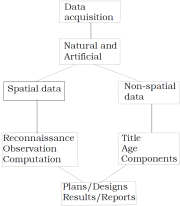
Figure 1. Research Flow Chat (source: field observation).

3.1. Equipment Used for Data Acquisition

The following equipment were used during the execution of the project

1. Differential GPS with its accessories

2. Steel tape (50m)

3. Short pegs

4. Writing materials

Reconnaissance exercise was done to acclimatize with the area using some instrument like tapes, cutlass and writing materials and found out some survey beacons (FPO/001 – FPO/008) well densified round the catchment area which were used as reference points for the research exercise. Road networking of the catchment area in conjunction with drainages in the area was well planned in terms of the road networking and drainage facilities. The width of all the road carriages was up to 3.2m. Also, the drainage facilities were well networked round the area which all terminated at the extreme low end of the catchment area leading into an averagely large water body. The catchment area had catchment pits of different sizes in width and depth built in strategic place round the area of study and the conditions of each catchment pits were checked. Plans and strategies on how the research was handled step by step base on the data gathered from the reconnaissance diagram so that nothing will be left untouched.

The survey instrument was set up, centered and leveled for observation on the base station FPO/007. The data was stored on the instrument internal memory drive/chip and later downloaded for processing on the computer system. The perimeter of the research area was traversed basically for coordinating the boundary points as the master receiver of the DGPS was stationed on the reference point. Synchronize the master’s receiver with the rover receiver to take observation on all selected points. The details taken within the catchment area are artificial features that have direct relation with the research e.g. buildings, roads, drainages, catchment pits, etc. Their coordinate values (northing, easting and height) of each feature were taken and saved on the instrument. The total spot heights of four hundred and fifty four (454) were picked for the topographic mapping. Each categories of feature on the area of study was given different identity for proper identification (i.e. ‘R’ after each road, ‘C’ after catchment pit, ‘B’ after buildings and ‘G’ after drainage).

3.2. Data Processing

This is the data processing where the acquired data stored in the memory of the instrument were downloaded into a personal computer system. The downloading was done with the aid of a downloading cable connected to link the computer system which have the software if the DGPS and the instrument. Thereafter, they were imported into the ArcGIS for plotting and to carry out spatial analysis. The area calculation as well as determining the bearing and distances were calculated using the Survey Word software for easy editing, analyzing, updating and retrieval.

The downloaded X, Y coordinates were separated according to the code used to identify the features in the instrument. This was copied to Microsoft Excel and it was edited. Check the appendix for the tables.

3.2.1. Back/Area Computation

After the completion of data processing on the computer system, the boundary point coordinates that is in Easting and Northing values of the study area were extracted and used for determining the latitude, departure, distance and bearing of the boundary line of the study area by using Survey Word software. The area computation was displayed using back computation method run by Survey Word through the back computation procedure. The total area of the research site was calculated to be 214320.650sq.m (21.432 Hectares).

3.2.2. Database Creation

Having completed the design phase, the next stage was the creation phase when the database tables were populated with the required spatial analysis possible. The representations of the data in the tables provide an easy way to visualize access and manipulate the information in the database.

3.3. Database Implementation

This involved the combination and storage of the graphic data in creating the database for the purpose of spatial analysis and query. The basic datasets were put in format as data acquired (x, y, z, coordinates) for each features were imported in to the ArcGIS 10.1 software.

3.3.1. Spatial Analysis

ArcGIS was used because of its spatial analytical capability especially; Queries, overlay operation, buffering, spatial search, topographic operation and neighborhood and connectivity operations. GIS uses this spatial analytical capability to answer fundamental generic question of location, condition, trend, routing, pattern and modeling by the manipulation and analysis of input data

[5]

. The major analyses performed in this research were queries, overlay operation and topographic operation.

It also has the ability to perform complex spatial analysis and modeling operations in support to environmental planning and mapping. Queries were designed for the purpose of retrieving information from the database. The queries performed in this research gave answers to certain generic questions asked from the database which were made possible as a result of the implicit link of both the spatial and attribute data. Queries may be single criterion or multiple criterions.

3.3.2. Composite Plan/Topographic Plan

It describes spatial information on any typical topographic plan. It shows well defined boundary, the contour lines and features (roads, building structures, catchment pits, etc) in the study area in Figure 2 below. The composite plan was made from overlay of contour map and detail map of the study area to produce the topographic map of the area which shows the relationship that exists between the various spatial entities in the study area

[6]

. This result can be used to determine area that is prone to erosion and how to control it.

Download: Download full-size image

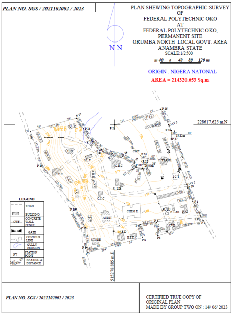
Figure 2. Topographic Composite Map.

3.3.3. Topographic Operation and Analysis

This operation was performed from digital elevation model generation using ArcGIS 10.1 version. The earth is 3-dimensional, most GIS application includes some element of 3-dimenstional analysis of which topographic operations and analysis of surface terrain becomes paramount

[12]

. Contour, Slope, Aspect and Digital Terrain Model (DTM) generations are considered as the most common uses in application of terrain model use in GIS. The analyses were performed using ArcGIS 10.1 version and products generated were:-

1. Buildings with pervious and impervious landscaping

2. Drainages that convey high and low flood in the area

3. Contour lines below and above 180m

4. Results

4.1. Application of Produced Topographic Map

The various topographic maps generated in this study can be used for planning purposes and decision making. The topographical map of Permanent Site, Federal Polytechnic, Oko, shows all the features as they exist on the ground and other available areas for future development. The generated topographical maps were used to further analyze in the area of study the Fluid Dynamics of flood that resulted into the gully erosion.

The contour line values on the topographic map was sectioned into two parts so to compute the steepness and flatness of the surface of the either sides in the catchment area. The steep side falls between the higher values of 192m to lower value of 182m contour lines on the map. Also, the gentle or flat side falls between the higher values of 180m and lower values of 172m contour lines on the map.

4.1.1. The Analysis on Steep Slope

For the analysis on steep side, the total length being scaled-off was up to 324.5m from the road R1b. The side was sectioned into six at 75m intervals on scale 1:2500. The height difference of the contour lines on map was designed at 2m interval. The space between the lines along each section was scaled-off and the values scaled-off from the topographic map contour lines were tabulated to compute the possible slope in-between those lines.

To calculate the slope values in-between the contour lines, slope formula was used;

= \sqrt ({a^{2} + b}^{2})

(1)

Table 1. The Analysis on Steep Slope.

Contour lines (m)	196-194	194-192	192-190	190-188	188-186	186-184	184-182
A-A (m)	10	8	7	6.5	7	9	12
Slope (m)	10.198	8.246	7.28	6.801	7.28	9.02	12.166
B-B (m)	12	8	10	5	5	4	4
Slope (m)	12.166	8.246	10.198	5.365	5.385	4.472	4.472
C-C (m)	10	9	8	8	11.5	18	16
Slope (m)	10.198	9.22	8.246	8.246	11.673	8.111	16.125
D-D (m)	10	8	7	8	13	26	19
Slope (m)	10.198	8.246	7.28	8.246	13.159	26.077	19.105
E-E (m)	10	8	8	6	6	6	8
Slope (m)	10.198	8.246	8.246	6.325	6.325	6.325	8.246
F-F (m)	16	10	9	8	10	11	12
Slope (m)	16.125	10.198	9.22	8.246	10.198	11.18	12.166

4.1.2. The Analysis on Gentle Slope

For the analysis on gentle or flat side, the total length of the side covered by the contour lines that were far apart was scaled-off and found out that it was up to 324.5m from the road R1b. The side was sectioned into six at 75m intervals on scale 1:2500. With the height difference of the contour lines on map designed at 2m interval. The space between the lines along each section was scaled-off. The values from the topographic map contour lines were tabulated to compute the possible slope in-between those lines on that side as well. Table 2 below shows the results.

To calculate the slope values in-between the contour lines, slope formula was used;

= \sqrt ({a^{2} + b}^{2})

(1)

After getting the values from the two types of slopes from the area, it was found out that there was a need to get the forces that were acting on the runoff in drainages on the either side of the road to know what really caused the gully erosion on the fact that infiltration on the steep slope side is very low compared to the gentle surface and also from the fact that new structures that were put in place on the steep area could have as well caused the increase in non-infiltration of water into the ground because those structures had impermeable landscape around them.

Table2. The Analysis on Gentle Slope.

Contour line	178-176	176-174	174-172
1-1	28	61	61
Slope (m)	28.089	29.069	61.033
2-2	21	34	50
Slope (m)	21.095	34.059	50.04
3-3	20	33	23
Slope (m)	20.1	33.061	23.087
4-4	16	37	31
Slope (m)	16.125	37.054	31.064
5-5	16	42	33
Slope (m)	16.125	42.048	33.061
6-6	32	30	38
Slope (m)	32.062	30.067	38.053

4.1.3. Comparison Between Analyses

From the two tables above (1 and 2), it can be deduced in the first table that the slope values are very high which will make the run-off on the side to quickly run down into the drainage with greater gravitational force been effected by the steepness of the slope which result to no infiltration and even wear away the surface of the ground. While on the other table, it can be deduced that the slope values are very low which will cause the run-off to take a long period of time to get to drainage due to the flatness of the side and resulting to having larger quantity of the run-off infiltrated into the ground

[14]

4.2. Fluid Dynamics

In view of checking the reason for the gully erosion, the impact of the flood flow was calculated from fluid dynamic’s equations to know how the erosion took place at drainage G7, though; it is the exit drainage that conveyed the flood into the river at the back of the study area. The fluid dynamics was computed to know the possible quantity of the energy exerted that pulled out the drainage (G7). Since all the drainage structures in the study area are open channels, in adopting the fluid mechanics equations, all the drainages were calculated based on their varying dimensions and also the fluid discharge into the drainage from the steep slope side of the catchment area and the fairly low surface of the study area. The depth of the gully erosion from the normal surface to the base was 14.63m deep as at the period of observation.

Hydro-Kinematics is the science that deals with the geometry of fluid flow without regarding the forces causing the motion. The fluid mechanics basic equations were used to compute the fluid dynamics of the area; i) continuity equation, ii) energy equation and iii) impulse-momentum equation

[16]

4.2.1. Continuity Computation

Specific time value of 5seconds was used to check on the rate of discharge at any point of the flood in the study area. The possible rate of flood discharge from the constructed drainages with the possible speed of the fluid flow in the drainage was calculated. The result is shown in Table 3 below. The rate of discharge is denoted with

Q = av

(2)

Q = area x average velocity

A = lb = length x breadth = m^{2}

(3)

V = d / t = distance / time = m / s

(4)

Table 3. The Analysis of the Continuity Equation.

SN	I.D	Depth (m)	Width (m)	Area (m²)	Distance (m)	Time (s)	Velocity (m/s)	Discharge (A/V)
1	R1a	0.6	0.6	0.36	156.3	5	31.26	11.254
2	R1b	0.6	0.6	0.36	82.05	5	16.41	5.908
3	G1	0.6	0.6	0.36	33.5	5	6.7	2.412
4	G2	0.5	0.8	4.00	87.5	5	17.5	7.000
5	G3	0.5	0.9	0.45	81.73	5	16.35	7.356
6	R2	1.2	1.0	1.2	216.31	5	43.262	51.914
7	R3a	0.6	0.6	0.36	122.64	5	24.528	8.83
8	R3b	0.6	0.6	0.36	100.49	5	20.98	7.235
9	R4a	0.7	0.7	0.49	179.92	5	35.984	17.632
10	R4b	0.6	0.6	0.36	97.82	5	19.564	7.043
11	G4	0.9	0.8	0.72	163.27	5	32.654	23.511
12	R5	0.9	0.8	0.72	152.31	5	30.465	21.933
13	R6	0.7	0.7	0.49	109.72	5	21.944	10.753
14	R7	0.7	0.7	0.49	132.52	5	16.565	8.117
15	R8	0.7	0.7	0.49	94.82	5	18.964	9.292
16	G5	0.9	0.8	0.72	63.46	5	12.692	9.138
17	G6	0.7	0.7	0.49	71.87	5	14.374	7.043
18	G7	1.5	1.2	1.8	32.61	5	6.552	11.739
19	R9	0.7	0.7	0.49	94.6	5	18.92	9.271

Discussion: It can be noticed that the discharge value at G7 is very great even at a shortest distance. This discharge is more than what the G7 drainage can carry which later collapsed and caused the gully erosion.

4.2.2. Energy Computation

In adopting the Bernoulli’s equation, the total energy dissipated by the fluid particles in motion states that “if an ideal incompressible fluid flow is steady and continuous, the sum of the potential energy, kinetic energy and pressure energy is constant in a stream line”. Total energy is denoted with H_T. The results are shown in table 4 below.

Total energyHt= z+

V^{2}

/2g+ρ/w (

Nm . kg of fluid)

(5)

Potential energy exists due to configuration or position above datum line and is denoted with z

Kinetic/velocity energy exists due to velocity of flowing fluid and is calculated with;

V^{2}

/2g(6)

Where v is the velocity due to gravity (g = 9.81), which gave us the work done by the molecular properties of the water movement through each drainage at a particular point in time. Base on this fact of work done by the flow, we can calculate the force that activates the movement.

Ek=F.d= work done(7)

Pressure energy exists due to the pressure of the fluid and is measured in

\frac{ρ}{w}

, where p is the pressure and w is the weight density of the liquid (Specific weight of water

= 9.81 kN m^{3}

P=F/A = (kN/m²)(8)

Table 4. The Analysis of the Energy Equation.

SN	I.D	Distance (m)	Velocity (m/s)	Area (m²)	Z	V²/2g	F	P (F/A)	E_p	H_T
1	R1a	156.3	31.26	0.36	1.14	49.81	0.31	0.86	0.0877	51.0377
2	R1b	82.05	16.41	0.36	0.94	13.73	0.17	0.47	0.0480	14.718
3	G1	33.5	6.7	0.36	1.15	2.29	0.07	0.19	0.014	3.4594
4	G2	87.5	17.5	4.00	0.83	15.61	0.18	0.45	0.0459	16.4859
5	G3	81.73	16.35	0.45	3.4	13.65	0.17	0.38	0.0387	17.0887
6	R2	216.31	43.262	1.2	7.36	96.2	0.44	0.37	0.0377	103.5977
7	R3a	122.64	24.528	0.36	1.5	30.66	0.25	0.69	0.0703	32.2303
8	R3b	100.49	20.98	0.36	0.6	20.59	0.20	0.56	0.0571	21.2471
9	R4a	179.92	35.984	0.49	2.81	66.00	0.37	0.76	0.0775	68.8875
10	R4b	97.82	19.564	0.36	0.82	19.51	0.20	0.56	0.0571	20.3871
11	G4	163.27	32.654	0.72	2.11	54.35	0.33	0.46	0.0469	56.5069
12	R5	152.31	30.465	0.72	1.83	47.30	0.31	0.43	0.0438	49.1738
13	R6	109.72	21.944	0.49	5.2	24.53	0.22	0.45	0.0459	29.7759
14	R7	132.52	16.565	0.49	1.2	13.99	0.11	0.22	0.0224	15.2124
15	R8	94.82	18.964	0.49	5.6	18.33	0.19	0.39	0.0398	23.9698
16	G5	63.46	12.692	0.72	1.72	8.21	0.13	0.18	0.0183	9.9483
17	G6	71.87	14.374	0.49	2.3	10.53	0.15	0.31	0.0316	12.8616
18	G7	32.61	6.552	1.8	0.52	2.17	0.07	0.04	0.0041	2.6941
19	R9	94.6	18.92	0.49	7.94	18.24	0.19	0.39	0.0398	26.2198

4.2.3. Impulse-Momentum Computation

The application of this equation leads to the solution of the problems of fluid mechanics which cannot be solved by energy principles alone but can be used in conjunction with the energy equation to obtain complete solution of engineering problems based on the law of conservation of momentum which states that “the net force acting on a mass of fluid is equal to change in momentum of flow per unit in that direction”. The result is shown in the Table 5 below.

F = ma

m = mass of the fluid

a = acceleration acting in the same direction as

F (

a=dv/dt)

Ft = mv(9)

Table 5. The Analysis of the Impulse/Momentum Equation.

SN	I.D	F	Time	F.t
1	R1a	0.31	5	1.55
2	R1b	0.17	5	0.85
3	G1	0.07	5	0.35
4	G2	0.18	5	0.90
5	G3	0.17	5	0.85
6	R2	0.44	5	2.2
7	R3a	0.25	5	1.25
8	R3b	0.20	5	1
9	R4a	0.37	5	1.85
10	R4b	0.20	5	1
11	G4	0.33	5	1.65
12	R5	0.31	5	1.55
13	R6	0.22	5	1.1
14	R7	0.11	5	0.55
15	R8	0.19	5	0.95
16	G5	0.13	5	0.65
17	G6	0.15	5	0.75
18	G7	0.07	5	0.35
19	R9	0.19	5	0.95

Discussion: This then showed that the net force acting on a mass of fluid at G7 over a period of time is equal to change in momentum of flow per unit in that direction which then pull off the drainage (G7) and if there is no check to reduce the quantity of water coming to this spot or construct another channel to support the G7 in conveying flood away from the catchment pit, the gully erosion will continue to widening.

4.3. Hydraulic Design of the Most Economical Drainage

From the topographic plans, these data were obtained for the hydraulic design for the most economical drainage system:

Area of the basin A = 214320.653m², Perimeter of the basin P = 2605.449m,

Length of the mainstream L = 1125.428m

Average width of the basin

W = \frac{A}{L} = \frac{214320.653}{1125.428}

= 190.435m(10)

To find compactness of the basin

Radius of equivalent area

R = \sqrt{\frac{A}{π}} = \sqrt{\frac{214320.653}{3.142}}

= 261.173m(11)

Circumference of the equivalent area = 2πR = 2 x 3.142 x 261.173 = 1641.214m

Factor of compactness

= \frac{P}{C} = \frac{2605.449}{1641.214}

=1.6(12)

Elongation ratioE_r

= \frac{2 R}{L} = \frac{2 x 261.173}{1125.428}

= 0.46(13)

Factor of area =

\frac{A}{L^{2}}

\frac{214320.653}{{1125.428}^{2}} =

0.17(14)

Difference in elevation between most remote points of the area

∆

H = 198 – 160 = 38m

Slope =

\frac{∆ H}{L}

\frac{38}{1125.428}

= 0.0338(15)

Time of concentrationt_c=

\frac{{0.0194 L}^{0.77}}{S^{0.385}}

\frac{{0.0194 x x 1125.428}^{0.77}}{{0.0338}^{0.385}}

= 15.99 = 16min.(16)

Rainfall intensityi=

\frac{T}{{(t + 10)}^{0.38}}

(17)

Let T = 50years

i =

\frac{50}{{(16 + 10)}^{0.38}}

\frac{50}{3.44897}

= 14.5m/hr

Q = 2.78

CiA

= 2.78

x 0.3 x 14.5 x 0.214320.653

= 2.55m³/s(18)

For most economical design of rectangular drainage using Manning formula

Q =

\frac{A}{n} ({R)}^{\frac{2}{3}} ({S)}^{\frac{1}{2}})

(19)

R =

\frac{y}{2}

and b =

2 y

S =

\frac{14.63}{150}

= 0.0953

n = 0.017

2.55 =

\frac{0.21432}{0.017} ({\frac{y}{2})}^{\frac{2}{3}} ({0.0953)}^{\frac{1}{2}}

\frac{y^{2 / 3} x 0.0661620801}{0.02669858179}

y^2/3=

\frac{2.55 x 0.02669858179}{0.0661620801}

= 1.04

y = 1.06 = 1.1m

b =

2 y

2 x 1.1

= 2.2m

velocity of flow in the drainage

v =

\frac{Q}{A}

\frac{Q}{(b x y)} = \frac{2.55}{(2.2) (1.1)}

= 1.1m/s(20)

v > 1

The velocity of the flow is more than the minimum value which shows that there will be less or no deposition of sediment in the drainage. The sketch of the drainage as designed is shown Figure 3 below.

Download: Download full-size image

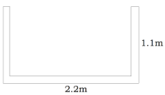
Figure 3. Diagram of the section from the designed drainage.

4.3.1. Structural Design of the Rectangular Drainage

Download: Download full-size image

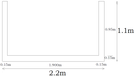
Figure 4. Structural design of the rectangular drainage.

Characteristics strength of concrete fcu = 25N/mm²

Characteristics strength of steel fy = 410N/mm²

Unit weight of concrete, Y_conc = 24kN/m³

Unit weight of soil, Y_soil = 15kN/m³

Angle of internal friction of soil = 2^o

Soil cohesion = 12.4kN/m²

unit weight of water Y_w = 9.81kN/m³

Design

Based on per meter length of basin,

Analysis is done for two conditions

When the drainage is empty

When the drainage is full of water

Effective height of earth retain = 950mm

Assume bar size = 16mm

Wall thickness =

\frac{H}{10}

\frac{950}{10}

= 95mm(21)

Add cover = 50mm

Add ½ bar size =

\frac{16}{2}

= 8mm

Wall thickness = 95 + 50 + 8 = 15.3mm

Table 6. Members analysis for the structural design.

H (m)	D_min (m)	d_min (mm)	Cover (mm)	½ bar	h (mm)
1.10	0.95	950	50	8	153

Try base thickness = 150mm = 0.15m

Try wall thickness = 150mm = 0.15m

Internal width = 1.9m

Case 1: Drainage Empty (Earth Pressure Acting)

Download: Download full-size image

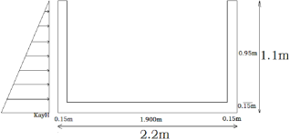
Figure 5. Case 1 structural design.

Lateral earth pressure, pa

Ka= tan^-1(45–

\frac{\emptyset}{2}

) = tan^-1(45–

\frac{18}{2}

) = 0.53(22)

pa=kax y xH = 0.53 x 18 x 1.1 = 10.49kNm(23)

Horizontal thrust Pa

Pa = ½ xkax y x H²= ½ x 0.53 x 18 x 1.1²= 5.8kN/m (24)

Moment due to horizontal thrust Ma

Ma = Pa x

\frac{H}{3}

= 5.77 x (

\frac{1.1}{3}

) = 2.12kN-m/m (25)

Ultimate moment Mu = 1.4Mu

1.42 x 2.12 = 2.97kN-m/m

Table 7. Summary of Case 1 bending moment analysis.

Ø	45 - Ø/2	Ka	y	H	H²	Pa	H/3	Ma
2⁰	0.53	0.53	18	1.1	1.21	5.8	0.3667	2.12

Base

Effective span, Le =bt(

\frac{t_{w}}{2} + \frac{t_{w}}{2}

) = 1.9 + (

\frac{0.15}{2} + \frac{0.15}{2}

) = 2.05(26)

Weight of side wall

w = hw x tw x yconc .

1.1 x 0.15 x 24

= 3.96 = 4kN/m(27)

Upward soil reaction at base

q =

\frac{2 w}{l_{e}}

\frac{2 (3.96)}{2.05}

= 3.86 = 3.9kN/m²(28)

Table 8. Summary of reactions on Case 1 members.

b (m)	Le (m)	h_w (m)	t_w (m)	Y_conc_.	load	W (kN/m)	2W	q (kN/m²)
1.9	2.05	1.1	0.15	24	4	3.96	7.92	3.9

Free peak bending moment at base M =

\frac{{ql}^{2}}{8}

(29)

M =

\frac{{3.9 x 1.21}^{2}}{8} =

0.71kN-m/m.(30)

Fixed bending moment

FEM at base from lateral earth pressure

FEM = 2.97kN-m/m

Net BM =M_net= Free BM – FEM.(31)

= 0.71 – 2.97 = -2.26kN-m/m

Ultimate net moment, M_net = 1.4M_net

1.4 x -2.26 = -3.16kN-m/m.(32)

Table 9. Case 1 Ultimate moment analysis.

Q	Le	Le²	M (kN-m/m)	FEM	M_net	MU_net
3.9	2.05	4.2025	0.71	2.97	-2.26	-3.16

Case 2: Drainage Full (Water Pressure Acting)

Download: Download full-size image

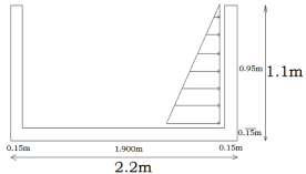
Figure 6. Case 2 structural design.

Loading on wall:

Depth of water = 0.95m

Water pressure, P_wk

P_w=y_w+ h = 9.81 x 0.95 = 9.32kN/m^2.(33)

Thrust due to water pressure, P_w

½ xy_wxh²= ½ x 9.81 x 0.95²= 4.43kN/m.(34)

Moment due to water Mw

M_w= P_wx

\frac{h}{3}

= 4.43 x

\frac{0.95}{3}

= 1.4kN-m/m(35)

Ultimate limit state MU_w

MU_w= 1.4 x 1.4 = 1.96kN-m/m. (36)

Table 10. Summary of Case 2 bending moment analysis.

y_w	H	P_w	h²	P_w	h/3	Mw	MUw
9.81	0.95	9.32	0.9025	4.43	0.3167	1.4	1.96

Base:

Weight of P_w

P_w=y_wx h x b = 9.81 x 0.95 x 1.9 = 17.71kN/m. (37)

Weight of wallsW_w

W_w=t_wxh_wxy_conc.X 2 = 6.84kN/m. (38)

Upward reaction at base q

q =

\frac{P_{w} + W_{w}}{L_{e}}

\frac{17.71 + 6.84}{2.05}

= 11.98kN/m^2.(39)

Table 11. Summary of reactions on Case 2 members.

Yw	h	B	Pw	tw	hw	Yconc.	Ww	Q
9.81	0.95	1.9	17.71	0.15	0.95	24	6.84	11.98

Free bending moment at base due to water BM

M =

\frac{{ql}^{2}}{8}

\frac{{11.98 x 0.9025}^{2}}{8}

= 1.22kN-m/m(40)

Free bending moment at base due to water pressure

FEM = 1.4kN-m/m

Net base at base Mnet = free Bm – FEM

= 1.22 – 1.4 = -0.18kN-m/m

Ultimate net moment, Mnet

MUnet = 1.4 x -0.18 = -0.25kN-m/m

Table 12. Case 2 Ultimate moment analysis.

Q	Le	Le²	M	FEM	Mnet	MUnet
11.98	0.95	0.9025	1.2	1.4	-0.18	-0.25

Table 13. Summary of Moment in Cases 1 and 2.

CASE	BENDING MOMENT AT WALL	BENDING MOMENT AT SPAN OF BASE
1	2.97	-3.16
2	1.96	-0.25

The wall will be designed for max bending moment

BM = 2.97kN-m/m

The base will be designed for max bending moment

BM = -3.16kN-m/m

Steel reinforcement

Wall

Max = 2.97kN-m/m

H = 150mm

Concrete cover = 50mm

Assumed bar size Ø = 16mm

Assumed width = 1000mm

d = h – cc - Ø/2 = 150 – 50 – 16/2 = 92mm(41)

K =

\frac{M}{(b d^{2} f_{cu})}

\frac{2.97 x 10^{6}}{(1000 x 92^{2} x 25)}

= 0.014(42)

K = 0.014 < 0.15

L_a= (0.5 + √0.014 –

\frac{k}{0.9}

)(43)

Use L_a= 0.95

Z = L_ax d = 0.95 x 92 = 87.4mm(44)

As req. =

\frac{M}{(0.87 x f_{y} x Z)}

(45)

\frac{2.97 x 10^{6}}{(0.87 x 410 x 87.4)}

= 95.27mm²/m

Use Y12 @ 300 (377mm²/m)

Distribution reinforcement

Min. steel = 0.13%bh= (0.13/100) x 1000 x 150 = 195mm²/m.(46)

Use Y10 @ 200mm (393mm²/m)

Table 14. Reinforcement distribution analysis.

M x 10⁶	Fy	0.87fy	Z	As req.	0.13%	b	h	Min steel
2.97	410	356.7	87.4	175.78	0.0013	1000	150	195

Bottom steel

Mmax= -3.16

H = 150mm

Conc. Cover cc = 50mm

Assume bar Ø = 16mm

Assume width = 2000

d = h – cc –

\frac{\emptyset}{2}

= 92. (47)

K =

\frac{M}{(b d^{2} f_{cu})}

\frac{- 3.16 x 10^{6}}{(2000 x 92^{2} x 25)}

= 0.007(48)

K = 0.007 < 0.15

Table 15. Analysis for 'k-value'.

H	Cc	Ø/2	d	M x 10⁶	b	d²	fcu	K
150	50	8	92	5.38	2000	8464	25	0.007

L_a= (0.5 + √0.007 –

\frac{k}{0.9}

)(49)

Use L_a= 0.95

Z = L_ax d = 0.95 x 92 = 87.4mm.(50)

As req. =

\frac{M}{(0.87 x f_{y} x Z)}

(51)

\frac{- 3.16 x 10^{6}}{(0.87 x 410 x 87.4)}

= -101.36

Distribution reinforcement as per wall

Top Steel

As = 101 x (

\frac{2.97}{3.16}

) = 95.27mm²/m.(52)

Use Y12 @ 300 (377mm²/m)

Table 16. Reinforcement distribution for the wall.

L_a	La	Z	Fy	M span (10⁶)	M support (10⁶)
k/0.9	√0.007 – $\frac{k}{0.9}$	87.4	410	2.97	-3.16

Download: Download full-size image

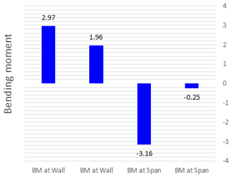
Figure 7. The bar chat of the bending moment.

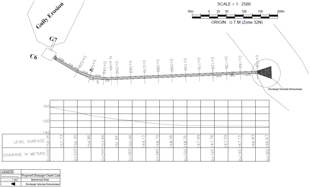
4.3.2. Summary of Design Outputs

The graph above displays a moment-by-moment summary for the above design. Following the determination of discharge Q, Mannings coefficient n, and channel slope s on the aforementioned design. The drainage size was proportioned using the discharge. The process for determining the drainage dimension for the drainage channel design involved first estimating the section factor, AR^2/3 in terms of the drainage width of flow, b, and its normal depth of flow, y, and then determining the normal depth by trial and error. To get the needed total depth of flow. The potential incidence of the loads was taken into account when calculating the bending moment. Generally speaking, these two factors were used to construct the drainage systems.

Drainage Empty: Earth Pressure Acting

Drainage Full: Water Pressure Acting

Because of the condition’s larger moment value caused by the action of lateral Earth pressure, case 1 analysis from the chart above was chosen for the design displays the output from the previous design.

4.3.3. Drainage Profile Design

The figure 8 below depicts the plan of the proposed designed drainage that will convey the flood from the catchment pit C6 to the river bank located at the back of the area of study. Three catchment pits were introduced in the design at strategic points along the drainage to step down the flow speed. The distance measured was 150.58m. Provision of this drainage system will provide solution to the erosion menace at that spot (G7).

Download: Download full-size image

Figure 8. The Plan, Traverse Lines and Profile. The Plan, Traverse Lines and Profile.

5. Conclusion

The level of damage caused by erosion in the permanent site, Federal polytechnic Oko, Anambra state was determined. The accuracy and functionality of this research rely on a large extent of the accuracy of topographical data and the computation of the discharge of flow on the ground surface and through the drainages. And above all this research has given me much needed experience in term of using topographic survey method in generating all the necessary data for analyzing and designing a most economical drainage. Also, the data generated from the geo-database aid in designing the selected structural members of the drainage system that control the flood and totally put an end to the erosion menace.

Abbreviations

DGPS	Differential Global Positioning System
EIA	Environmental Impact Assessment
R	Road
C	Catchment Pit
B	Buildings
G	Drainage
DTM	Digital Terrain Model

Conflicts of Interest

The authors declare no conflicts of interest.

References

[1]	Agor R. (2012), [Formerly Officer Survey of India], Formerly, Lecturer in Civil Engineering, Technical Education, Delhi. Eleventh edition Romesh Chander Khanna, for KHANNA PUBLISHERS, NaiSarak, Delhi.
[2]	Constantine Mbajiorgu (2020) Assessment of surface water hydrology, Eco-Hydrological Systems Research Unit, Dept of Agricultural &Bioresources Engineering University of Nigeria, Nsukka.
[3]	Hatt B. E, Fletcher T. D, Walsh C. J, Taylor S. L (2004) The influence of urban density and drainage infrastructure on the concentrations and loads of pollutants in small streams. Environ Manage 34: 112–124.
[4]	Heer and Hagerty, (2006). Solid Waste Management, Publisher: Van Nostrand Reinhold Company, 1973: Original from: the University of California.
[5]	AI and LinkedIn community (2023). How do you use GIS and remote sensing tools for environmental impact assessment? Published on Mar. 13, 2023.
[6]	Banister and Raymond (2020). Surveying, The latest edition, fully revised and updated to reflect the changing nature of the subject and its technology, amazon. in/Surveying-Bannister/dp/0582302498.
[7]	Hassan Mahani, Geoffrey Thyne, (2023), Low-salinity (Enhanced) Waterflooding in Carbonate reservoirs in Recovery Improvement, 2023.
[8]	Sean C. (2021). Frontiers in Ecology and the Environment Reviews Open Access Trends in ecology and conservation over eight decades. Published by esajournals. Online library.wiley.
[9]	Vladimir Vishnyakov, EldarZeynalov, (2020), Oil recovery stages and methods, in Primer on Enhanced Oil Recovery, research publication, 2020.
[10]	Conner M. et al (2022): Methods for ecological research on terrestrial small mammals. Published on researchgate
[11]	Mohammad Ali Ahmadi, (2018), Waterflooding in Fundamentals of Enhanced Oil and Gas Recovery from Conventional and Unconventional Reservoirs, 2018.
[12]	Koorosh G. and Christina S. (2017) GIS as a vital tool for Environmental Impact Assessment and Mitigation. Published under licence by IOP Publishing Ltd, IOP Conference Series: Earth and Environmental Science, Volume 127, 2017, Toronto, Canada
[13]	Abdus Satter, Ghulam M. Iqbal, (2016), Waterflooding and waterflood surveillance in Reservoir Engineering, journal publication, 2016.
[14]	Pu and Li (2016) saturated cores through a core-holder by first flooding brine, article by sciencedirect, S0920410522010373.
[15]	James J. Sheng, (2020), Water injection, in Enhanced Oil Recovery in Shale and Tight Reservoirs, Journal Publication, 2020.
[16]	Eme L. C. (2016). Fluid Mechanics and Hydraulics, first edition text book, department of civil engineering, Chukwuemeka Odumegwu Ojukwu university, Uli, Publisher: Lumos Nig. Ltd.

Cite This Article

Plain Text BibTeX RIS

APA Style

Ogundeji, A. F., Nnamdi, E. C. (2024). Ecological Impact Assessment of Permanent Site of Federal Polytechnic Oko Using Topographic Survey Method. American Journal of Applied Mathematics, 12(5), 183-199. https://doi.org/10.11648/j.ajam.20241205.18

Copy | Download

ACS Style

Ogundeji, A. F.; Nnamdi, E. C. Ecological Impact Assessment of Permanent Site of Federal Polytechnic Oko Using Topographic Survey Method. Am. J. Appl. Math. 2024, 12(5), 183-199. doi: 10.11648/j.ajam.20241205.18

Copy | Download

AMA Style

Ogundeji AF, Nnamdi EC. Ecological Impact Assessment of Permanent Site of Federal Polytechnic Oko Using Topographic Survey Method. Am J Appl Math. 2024;12(5):183-199. doi: 10.11648/j.ajam.20241205.18

Copy | Download

@article{10.11648/j.ajam.20241205.18,
  author = {Ayodele Femi Ogundeji and Ezugwu Charles Nnamdi},
  title = {Ecological Impact Assessment of Permanent Site of Federal Polytechnic Oko Using Topographic Survey Method
},
  journal = {American Journal of Applied Mathematics},
  volume = {12},
  number = {5},
  pages = {183-199},
  doi = {10.11648/j.ajam.20241205.18},
  url = {https://doi.org/10.11648/j.ajam.20241205.18},
  eprint = {https://article.sciencepublishinggroup.com/pdf/10.11648.j.ajam.20241205.18},
  abstract = {Topographic survey based ecological impact assessment provides a mechanism for data integration, development, management and output presentation in a spatial environment. This research involved incorporating spatial data of all salient points at the Permanent Site of Federal Polytechnic, Oko, Anambra state to find a solution to the erosion menace. Differential Global Positioning System (DGPS) receiver was used to acquire spatial data of buildings, roads, spot height, drainages, catchment pits, etc. The topographic data were processed using ArcGIS software to analyze and produce the topographic maps. Presentations from the topographic survey revealed that the catchment topography runs between 160m – 198m height above the datum, the total area of the catchment area being 216320.653m2, perimeter is 2604.449m and the length of the mainstream is 1125.428m. Topographic maps of the area were used to assess the impact of the ecology on the area of study by analyzing the built up area, surface roughness, impervious and pervious surfaces. Hydraulic design of the drainage using best hydraulic section principle for most economic section to carry the flow was determined to solve the erosion problems in the catchment area. The flow rate obtained was 2.55m3/s and dimensions of the channel to be 1.1m depth and 2.2m width. The design of the selected structural members was done to mitigate against the erosion menace in the study area.
},
 year = {2024}
}

Copy | Download

TY  - JOUR
T1  - Ecological Impact Assessment of Permanent Site of Federal Polytechnic Oko Using Topographic Survey Method

AU  - Ayodele Femi Ogundeji
AU  - Ezugwu Charles Nnamdi
Y1  - 2024/10/18
PY  - 2024
N1  - https://doi.org/10.11648/j.ajam.20241205.18
DO  - 10.11648/j.ajam.20241205.18
T2  - American Journal of Applied Mathematics
JF  - American Journal of Applied Mathematics
JO  - American Journal of Applied Mathematics
SP  - 183
EP  - 199
PB  - Science Publishing Group
SN  - 2330-006X
UR  - https://doi.org/10.11648/j.ajam.20241205.18
AB  - Topographic survey based ecological impact assessment provides a mechanism for data integration, development, management and output presentation in a spatial environment. This research involved incorporating spatial data of all salient points at the Permanent Site of Federal Polytechnic, Oko, Anambra state to find a solution to the erosion menace. Differential Global Positioning System (DGPS) receiver was used to acquire spatial data of buildings, roads, spot height, drainages, catchment pits, etc. The topographic data were processed using ArcGIS software to analyze and produce the topographic maps. Presentations from the topographic survey revealed that the catchment topography runs between 160m – 198m height above the datum, the total area of the catchment area being 216320.653m2, perimeter is 2604.449m and the length of the mainstream is 1125.428m. Topographic maps of the area were used to assess the impact of the ecology on the area of study by analyzing the built up area, surface roughness, impervious and pervious surfaces. Hydraulic design of the drainage using best hydraulic section principle for most economic section to carry the flow was determined to solve the erosion problems in the catchment area. The flow rate obtained was 2.55m3/s and dimensions of the channel to be 1.1m depth and 2.2m width. The design of the selected structural members was done to mitigate against the erosion menace in the study area.

VL  - 12
IS  - 5
ER  -

Copy | Download

Author Information

Ayodele Femi Ogundeji

Surveying and Geoinformatics Department, Federal Polytechnic Oko, Oko Town, Nigeria

Contact Email

http://orcid.org/0009-0000-3571-6517
Ezugwu Charles Nnamdi

Civil Engineering Department, Alex Ekwueme Federal University Ndufu Alike, Abakaliki, Nigeria

Contact Email

http://orcid.org/0000-0002-5999-8536

Download PDF

Plain Text BibTeX RIS

APA Style

Ogundeji, A. F., Nnamdi, E. C. (2024). Ecological Impact Assessment of Permanent Site of Federal Polytechnic Oko Using Topographic Survey Method. American Journal of Applied Mathematics, 12(5), 183-199. https://doi.org/10.11648/j.ajam.20241205.18

Copy | Download

ACS Style

Ogundeji, A. F.; Nnamdi, E. C. Ecological Impact Assessment of Permanent Site of Federal Polytechnic Oko Using Topographic Survey Method. Am. J. Appl. Math. 2024, 12(5), 183-199. doi: 10.11648/j.ajam.20241205.18

Copy | Download

AMA Style

Ogundeji AF, Nnamdi EC. Ecological Impact Assessment of Permanent Site of Federal Polytechnic Oko Using Topographic Survey Method. Am J Appl Math. 2024;12(5):183-199. doi: 10.11648/j.ajam.20241205.18

Copy | Download

@article{10.11648/j.ajam.20241205.18,
  author = {Ayodele Femi Ogundeji and Ezugwu Charles Nnamdi},
  title = {Ecological Impact Assessment of Permanent Site of Federal Polytechnic Oko Using Topographic Survey Method
},
  journal = {American Journal of Applied Mathematics},
  volume = {12},
  number = {5},
  pages = {183-199},
  doi = {10.11648/j.ajam.20241205.18},
  url = {https://doi.org/10.11648/j.ajam.20241205.18},
  eprint = {https://article.sciencepublishinggroup.com/pdf/10.11648.j.ajam.20241205.18},
  abstract = {Topographic survey based ecological impact assessment provides a mechanism for data integration, development, management and output presentation in a spatial environment. This research involved incorporating spatial data of all salient points at the Permanent Site of Federal Polytechnic, Oko, Anambra state to find a solution to the erosion menace. Differential Global Positioning System (DGPS) receiver was used to acquire spatial data of buildings, roads, spot height, drainages, catchment pits, etc. The topographic data were processed using ArcGIS software to analyze and produce the topographic maps. Presentations from the topographic survey revealed that the catchment topography runs between 160m – 198m height above the datum, the total area of the catchment area being 216320.653m2, perimeter is 2604.449m and the length of the mainstream is 1125.428m. Topographic maps of the area were used to assess the impact of the ecology on the area of study by analyzing the built up area, surface roughness, impervious and pervious surfaces. Hydraulic design of the drainage using best hydraulic section principle for most economic section to carry the flow was determined to solve the erosion problems in the catchment area. The flow rate obtained was 2.55m3/s and dimensions of the channel to be 1.1m depth and 2.2m width. The design of the selected structural members was done to mitigate against the erosion menace in the study area.
},
 year = {2024}
}

Copy | Download

TY  - JOUR
T1  - Ecological Impact Assessment of Permanent Site of Federal Polytechnic Oko Using Topographic Survey Method

AU  - Ayodele Femi Ogundeji
AU  - Ezugwu Charles Nnamdi
Y1  - 2024/10/18
PY  - 2024
N1  - https://doi.org/10.11648/j.ajam.20241205.18
DO  - 10.11648/j.ajam.20241205.18
T2  - American Journal of Applied Mathematics
JF  - American Journal of Applied Mathematics
JO  - American Journal of Applied Mathematics
SP  - 183
EP  - 199
PB  - Science Publishing Group
SN  - 2330-006X
UR  - https://doi.org/10.11648/j.ajam.20241205.18
AB  - Topographic survey based ecological impact assessment provides a mechanism for data integration, development, management and output presentation in a spatial environment. This research involved incorporating spatial data of all salient points at the Permanent Site of Federal Polytechnic, Oko, Anambra state to find a solution to the erosion menace. Differential Global Positioning System (DGPS) receiver was used to acquire spatial data of buildings, roads, spot height, drainages, catchment pits, etc. The topographic data were processed using ArcGIS software to analyze and produce the topographic maps. Presentations from the topographic survey revealed that the catchment topography runs between 160m – 198m height above the datum, the total area of the catchment area being 216320.653m2, perimeter is 2604.449m and the length of the mainstream is 1125.428m. Topographic maps of the area were used to assess the impact of the ecology on the area of study by analyzing the built up area, surface roughness, impervious and pervious surfaces. Hydraulic design of the drainage using best hydraulic section principle for most economic section to carry the flow was determined to solve the erosion problems in the catchment area. The flow rate obtained was 2.55m3/s and dimensions of the channel to be 1.1m depth and 2.2m width. The design of the selected structural members was done to mitigate against the erosion menace in the study area.

VL  - 12
IS  - 5
ER  -

Copy | Download