Modelling and Simulation of a 3-D Reservoir for Enhanced Oil Recovery of ‘X’ Field in the Niger Delta Using Eclipse Software

Ihekoronye Kingsley Kelechi; Milton Roy Zwalatha; Caleb Abdullahi Ibrahim; Mohammed Hussein

doi:doi:10.11648/j.ajmcm.20240903.11

Research Article |

| Peer-Reviewed

Modelling and Simulation of a 3-D Reservoir for Enhanced Oil Recovery of ‘X’ Field in the Niger Delta Using Eclipse Software

Ihekoronye Kingsley Kelechi^*

, Milton Roy Zwalatha, Caleb Abdullahi Ibrahim, Mohammed Hussein

Published in American Journal of Mathematical and Computer Modelling (Volume 9, Issue 3)

Received: 8 January 2024 Accepted: 24 January 2024 Published: 30 August 2024

Views: Downloads:

Download PDF

Share This Article

Twitter
Linked In
Facebook

Abstract

Surfactant-polymer flooding is a tertiary enhanced oil recovery method used to recover oil that remained in the reservoir after the primary and secondary oil recovery mechanisms. Predicting the pressure in the reservoir is important for oil production as pressure changes with time. A suitable approach to achieve this task is to derive fluid flow equation based on the reservoir characteristics and solve them numerically which provide the solution to the mathematical fluid flow model (diffusivity equation). In this study, 3-D reservoir was modelled using Eclipse software. The fluid flow equations in a porous media were derived based on the simulated model and the reservoir conditions. Numerical solution using implicit formulation to solve the mathematical fluid flow model (diffusivity equation) was investigated by developing Python codes using Jupyter library to ascertain the pressure distribution for the reservoir and imported into Eclipse simulator. Simulation was carried out using surfactant-polymer and reservoir properties to determine the oil recovery. The results of the study showed that pressure increases with time as oil production continued, and water saturation decreased for the grid-cells of the reservoir. Waterflooding had oil recovery of 38.0% and water-cut of 59.0%, while surfactant flooding had oil recoveries of 42.0%, 46.5%, 49.0% and water-cut of 57.0%, 51.0%, 46.3%. In addition, polymer flooding had oil recoveries of 44.3%, 48.4%, 54.0% and water-cut of 50.0%, 45.0% and 33.0% respectively at different concentrations of 0.3%wt. 0.4%wt. and 0.5%wt.

Published in	American Journal of Mathematical and Computer Modelling (Volume 9, Issue 3)
DOI	10.11648/j.ajmcm.20240903.11
Page(s)	54-67
Creative Commons	This is an Open Access article, distributed under the terms of the Creative Commons Attribution 4.0 International License (http://creativecommons.org/licenses/by/4.0/), which permits unrestricted use, distribution and reproduction in any medium or format, provided the original work is properly cited.
Copyright	Copyright © The Author(s), 2024. Published by Science Publishing Group

Keywords

Python Software, Eclipse Software, Modelling, Surfactant-Polymer Flooding

1. Introduction

The demand for energy is increasing and oil reserve is steadily declining. There is need to increase oil production using surfactant-polymer flooding to meet up the energy demand

[4]

. Tertiary recovery method is the application of surfactant and polymer into the reservoir when the secondary technique had reached its economy limit (low oil recovery)

[9]

. Secondary oil recovery method can produce about 30% of the original oil in place

[1]

. The remaining oil left in the reservoir nearly 70% of the oil reserve can be recovered through the tertiary recovery methods especially as the global energy demand is growing rapidly

[8]

. Tertiary oil recovery is the application of chemicals in form of polymer and surfactant into the reservoir to recover additional oil that remained in the reservoir after primary and secondary recovery methods

[2]

Reservoir simulation using Eclipse software helps to predict the production history of the reservoir in the future in order to evaluate its oil recovery efficiency and understand the flow behavior of fluids during surfactant-polymer flooding processes

[6, 11]

. Forecasting of oil production from the reservoir using Eclipse software is very important to evaluate the performance of the well in the future

[10, 13]

. Simulation using chemical flooding are often used in the industry to optimize, design, and interpret the mechanisms of surfactant-polymer flooding methods

[5]

. Eclipse reservoir simulation are used for surfactant-polymer flooding, history matching and field oil performance

[12]

. Therefore, the focus of this study is to model a 3-D reservoir, obtain the pressure distribution of the reservoir by implicit formulation and simulate flow for surfactant-polymer flooding using Eclipse software.

2. Mathematical Fluid Flow Model

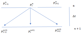
The development of a reservoir simulation begins with implicit/explicit formulation model (finite difference) for the mathematical fluid flow model (diffusivity equations) governing fluid flow in a porous media

[3]

. The diffusivity equation in form of partial differential equation describes the fluid flow in a porous medium and reservoir flow conditions

[14]

. Partial differential equation obeys the continuity equation, Darcy’s law and equation of state

[7]

3. Research Methodology

1) Develop a static and dynamic reservoir model.

2) Derive a mathematical model (diffusivity equation) that describes the simulated model.

3) Solve the mathematical model (diffusivity equation) in a discretize form using a PYTHON codes (Jupyter library) to obtain the pressure distribution and water saturation of the reservoir.

4) Simulate flow with surfactant-polymer flooding.

4. Static Reservoir Model

Download: Download full-size image

Figure 1. Reservoir Grid-blocks.

Table 1. Reservoir Rock and Fluid Properties.

Reservoir properties	Values
Grid-block dimensions (x, y, z)	Δx = 250 ft, Δy = 50 ft, Δz = 25 ft
Oil viscosity ( $μ)$	1.2 cP
Porosity ( $\emptyset)$	0.25
Permeability ( $K_{x}$ )	0.010 Darcy
Oil Formation Volume Factor, ${(B}_{o}$ )	1.12 rb/stb
Total Compressibility, ( $C_{t}$ )	0.0000035 ${psi}^{- 1}$
Initial Reservoir Pressure, ( $P_{i}$ )	3225 psia

4.1. Equation Governing Flow of Fluids in a Porous Media

The fluid flow in a porous media is governed by the continuity equation (material balance), transport equation (Darcy equation), and equation of state (slightly compressible fluids).

Continuity Equation (Material balance)

\frac{d}{dx} (gρ)

\frac{dp}{dt} A . \emptyset

(accumulating system)(1)

Transport equation (Darcy law)

V =

\frac{q}{A}

Q = VA(2)

Putting equation 1 into equation 2

\frac{d}{dx} (Vρ)_{A}

A . \emptyset \frac{dp}{dt}

\frac{d}{dx} (Vρ)

\emptyset \frac{dp}{dt}

(3)

Equation of state (slightly incompressible fluid)

Q =

\frac{k}{u} . \frac{dp}{dx}

(4)

Put equation 3 into 4

\frac{d}{dx} [\frac{kρ}{μ} \frac{dp}{dx}]

\emptyset \frac{dp}{dt}

(5)

\frac{d^{2} p}{d x^{2}} = \frac{u \emptyset c}{k} . \frac{dp}{dt}

(6)

Equation 6 is called the diffusivity equation for linear system

Where p = pressure in (psi)

U = viscosity in (cp)

\emptyset

= porosity dimensionless

C = compressibility in (psi)

K = permeability in (mD)

4.2. Basic Assumptions Used

1) One dimensional flow

2) Uniform grid system

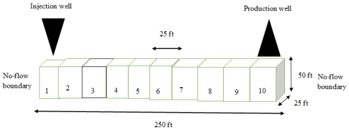
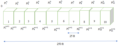
3) No-flow reservoir boundary condition

4) Homogeneous reservoir with block-centered grid cell

4.3. Finite Difference (Implicit Formulation)

Implicit Formulation

\frac{dp}{dt} = \frac{d^{2} p}{d x^{2}}

(7)

Download: Download full-size image

Figure 2. Implicit Formulation.

p_{i}^{n + 1}

p_{i}^{n}

\frac{∆ t}{{∆ x}^{2}} [p_{i + 1}^{n + 1} + p_{i - 1}^{n + 1} - 2 p_{i}^{n + 1}]

(8)

p_{i}^{n}

\frac{∆ t}{{∆ x}^{2}} p_{i + 1}^{n + 1}

\frac{∆ t}{{∆ x}^{2}} p_{i - 1}^{n + 1}

- 2

(\frac{∆ t}{∆ x^{2}}) p_{i}^{n + 1} - p_{i}^{n + 1}

(9)

\frac{{∆ x}^{2}}{∆ t} p_{i}^{n} = - p_{i + 1}^{n + 1} - p_{i - 1}^{n + 1} + 2 . p_{i}^{n + 1} + \frac{∆ x}{∆ t} p_{i}^{n + 1}

(10)

(\frac{{∆ x}^{2}}{∆ t}) p_{i}^{n} = (2 + \frac{{∆ x}^{2}}{∆ t}) p_{i}^{n + 1} - p_{i + 1}^{n + 1} - p_{i - 1}^{n + 1}

(11)

p_{i - 1}^{n + 1}

–

(2 + \frac{{∆ x}^{2}}{∆ t}) p_{i}^{n + 1} + p_{i + 1}^{n + 1} = - (\frac{{∆ x}^{2}}{∆ t}) p_{i}^{n}

(12)

For 10 grid blocks

Download: Download full-size image

Figure 3. Reservoir Grid block.

i = 1 and

p_{1}

= fixed boundary = 3225 psi

i = 10 and

p_{11}

= fixed boundary = 2000 psi

i = 2

p_{1}^{n + 1} - (2 + \frac{{∆ x}^{2}}{∆ t}) p_{2}^{n + 1} + p_{3}^{n + 1} = - (\frac{{∆ x}^{2}}{∆ t}) p_{2}^{n}

(13)

i = 3

p_{2}^{n + 1} - (2 + \frac{{∆ x}^{2}}{∆ t}) p_{3}^{n + 1} + p_{4}^{n + 1} = - (\frac{{∆ x}^{2}}{∆ t}) p_{3}^{n}

(14)

i = 4

p_{3}^{n + 1} - (2 + \frac{{∆ x}^{2}}{∆ t}) p_{4}^{n + 1} + p_{5}^{n + 1} = - (\frac{{∆ x}^{2}}{∆ t}) p_{4}^{n}

(15)

i = 5

p_{4}^{n + 1} - (2 + \frac{{∆ x}^{2}}{∆ t}) p_{5}^{n + 1} + p_{6}^{n + 1} = - (\frac{{∆ x}^{2}}{∆ t}) p_{5}^{n}

(16)

Therefore, for i =10, we have

i =10

p_{9}^{n + 1} - (2 + \frac{{∆ x}^{2}}{∆ t}) p_{10}^{n + 1} + p_{11}^{n + 1} = - (\frac{{∆ x}^{2}}{∆ t}) p_{10}^{n}

(17)

Since,

p_{1}^{n + 1}

p_{1}

= fixed

p_{11}^{n + 1}

p_{11}

= fixed

- (2 + \frac{{∆ x}^{2}}{∆ t}) p_{2}^{n + 1} + p_{3}^{n + 1} = - (\frac{{∆ x}^{2}}{∆ t}) p_{2}^{n} - p_{1}

(18)

p_{9}^{n + 1} - (2 + \frac{{∆ x}^{2}}{∆ t}) p_{10}^{n + 1} = - (\frac{{∆ x}^{2}}{∆ t}) p_{10}^{n} - p_{11}^{n}

(19)

Set -

(2 + \frac{{∆ x}^{2}}{∆ t})

(20)

[\begin{matrix} a_{11} & 1 & 0 & 0 & 0 & 0 & 0 & 0 & 0 \\ 0 & a_{22} & 1 & 0 & 0 & 0 & 0 & 0 & 0 \\ 0 & 1 & a_{33} & 1 & 0 & 0 & 0 & 0 & 0 \\ 0 & 0 & 1 & a_{44} & 1 & 0 & 0 & 0 & 0 \\ 0 & 0 & 0 & 1 & a_{55} & 0 & 0 & 0 & 0 \\ 0 & 0 & 0 & 0 & 1 & a_{66} & 0 & 0 & 0 \\ 0 & 0 & 0 & 0 & 0 & 1 & a_{77} & 0 & 0 \\ 0 & 0 & 0 & 0 & 0 & 0 & 1 & a_{88} & 0 \\ 0 & 0 & 0 & 0 & 0 & 0 & 0 & 1 & a_{99} \end{matrix}] [\begin{matrix} p_{2}^{n + 1} \\ p_{3}^{n + 1} \\ p_{4}^{n + 1} \\ p_{5}^{n + 1} \\ p_{6}^{n + 1} \\ p_{7}^{n + 1} \\ p_{8}^{n + 1} \\ p_{9}^{n + 1} \end{matrix}]

[\begin{matrix} - (\frac{{∆ x}^{2}}{∆ t}) p_{2}^{n} \\ - (\frac{{∆ x}^{2}}{∆ t}) p_{3}^{n} \\ - (\frac{{∆ x}^{2}}{∆ t}) p_{4}^{n} \\ - (\frac{{∆ x}^{2}}{∆ t}) p_{5}^{n} \\ - (\frac{{∆ x}^{2}}{∆ t}) p_{6}^{n} \\ - (\frac{{∆ x}^{2}}{∆ t}) p_{7}^{n} \\ - (\frac{{∆ x}^{2}}{∆ t}) p_{8}^{n} \\ - (\frac{{∆ x}^{2}}{∆ t}) p_{9}^{n} \\ - (\frac{{∆ x}^{2}}{∆ t}) p_{10}^{n} \\ - (\frac{{∆ x}^{2}}{∆ t}) p_{11}^{n} \end{matrix}]

(21)

Equation 21 in matrix form, was solved using Python codes (Jupyter library).

5. Dynamic Model

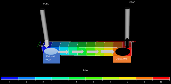
The reservoir was modelled using 3-dimensional method for a linear fluid flow system (figure 4). It contained three layers in X, Y, Z grids blocks which is 10 × 1 × 1 cells. The dimensions of the grid blocks are 250 ft in X direction while Z was 25 ft and Y direction was 50 ft. Each grid block was 25 ft respectively. The injection well was placed at 1 and 2 grid-blocks at the water zones, while the production well was placed at 9 and 10 grid blocks saturated with oil. The properties of the reservoir such as porosity, permeability, depth, and net to gross thickness were designed to model the linear flow reservoir. The reservoir grids defined the geometry and boundaries of the reservoir in the I, J and K directions. The aim of injecting the polymer is to increase the viscosity of water and control water mobility rate while the surfactant flooding changes the wettability of the rock from oil-wet to water-wet fluids to improve oil recovery. The simulation of oil production from the reservoir lasted for 11000 days. Waterflooding (secondary recovery method) was used as a base case to investigate the ultimate oil recovery before the introduction of surfactant and polymer as a tertiary oil recovery mechanism. Polymer and surfactant injection started at the first day of oil production. However, the surfactant used was formulated from Thevetia Peruviana seed oil via saponification reaction, while the polymer used was Gum Arabic. The properties of the characterized surfactant and polymer was inputted into the ECLIPSE software to evaluate the performance of the surfactant and polymer in enhanced oil recovery (EOR).

Download: Download full-size image

Figure 4. Reservoir Grid-blocks (3-D dynamic Model).

6. Results and Discussions

Results of the Implicit Formulation for Pressure Distribution and Water Saturation.

Download: Download full-size image

Figure 5. Pressure Distribution against time.

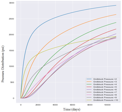
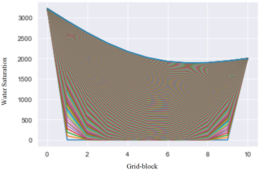
Figure 5 showed the pressure distribution of the reservoir (grid-blocks). Pressure increases with respect to time for each of the grid-blocks. Figure 6 showed the water saturation function of the grid blocks. The graph means that as the pressure in the reservoir increases as oil production continues, the water saturation decreases. The oil will fill the void space in the reservoir which was saturated with oil at each grid-blocks.

Download: Download full-size image

Figure 6. Water Saturation against Grid-block.

6.1. Results for Waterflooding

Download: Download full-size image

Figure 7. Field Oil Efficiency (oil recovery) against Time (days) for Waterflooding.

Download: Download full-size image

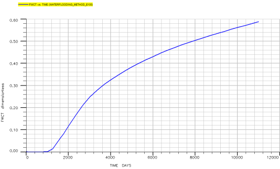
Figure 8. Field Water Cut (FWCT) against Time (days) for Waterflooding.

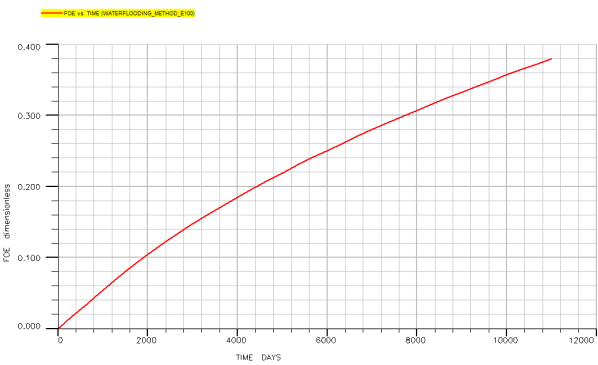
Figure 7 showed that the oil recovery was 38% when water was injected into the well to maintain reservoir pressure and enhance the reservoir sweep efficiency. The oil recovery result suggests that there is more oil that remained in the reservoir untapped since the saturated oil in this reservoir was 0.8 (80%). Therefore, tertiary recovery method using polymer/surfactant can be introduced in this reservoir to recover more oil. Figure 8, showed that water was delayed to nine hundred days before the field began to experience early water breakthrough. The reservoir water cut was very high (59 %), which showed that there will be high production of water in a short time from the well.

6.2. Results for Surfactant Flooding

Download: Download full-size image

Figure 9. Field Oil Efficiency (oil recovery) against Time (days) for Surfactant Concentration (0.3%wt.).

Download: Download full-size image

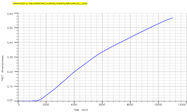
Figure 10. Field Water Cut (FWCT) against Time (days) for Surfactant Concentration (0.3%wt).

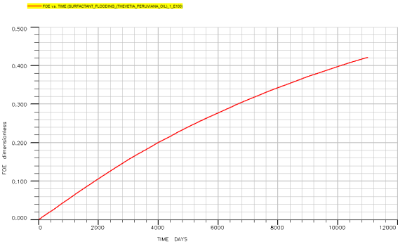
Surfactant flooding of 0.3% wt. gave oil recovery of 42% after eleven thousand days of oil production (figure 9). Increased in oil recovery using surfactant is due to the change in reservoir wettability from oil-wet to water-wet. The reservoir started producing water at one thousand, eight hundred days and field water cut was 57% (figure 10).

Download: Download full-size image

Figure 11. Field Oil Efficiency (oil recovery) against Time (days) for Surfactant Concentration (0.4%wt.).

Download: Download full-size image

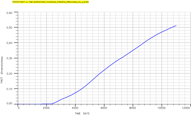
Figure 12. Field Water Cut (FWCT) against Time (days) for Surfactant Concentration (0.4%wt.).

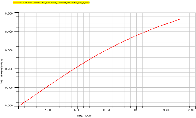
Oil recovery increased further to 46% at surfactant concentration of 0.4%wt. (figure 11). More so, the reservoir started producing water in two thousand, three hundred days as field water cut was observed to be 51% (figure 12).

Download: Download full-size image

Figure 13. Field Oil Efficiency (oil recovery) against Time (days) for Surfactant Concentration (0.5%wt.).

Download: Download full-size image

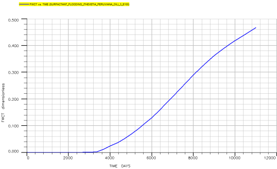
Figure 14. Field Water Cut (FWCT) against time (days) for Surfactant Concentration (0.5%wt.).

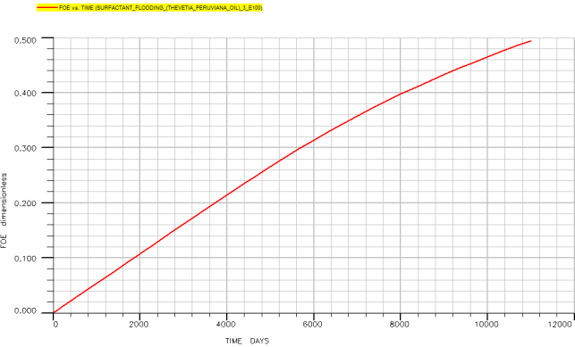
In figure 13, there was increase in oil recovery to 49% at surfactant concentration of 0.5%wt. The result means that concentration has a positive effect in surfactant flooding. It can be observed from the graph that this concentration gave the highest oil recovery when compared to 0.3%wt. and 0.4%wt. surfactant concentration respectively. Surfactant flooding recovered 49% of the total oil in place 80%. Water-cut was 46.3% that is the percentage of water in the fluid produced from the well (figure 14). Water production started from three thousand seven hundred days, which suggest that water was delayed as oil was produced from the reservoir.

6.3. Results for Polymer Flooding

Download: Download full-size image

Figure 15. Field Oil Efficiency (oil recovery) against Time (days) for Polymer Concentration (0.3% wt.).

Download: Download full-size image

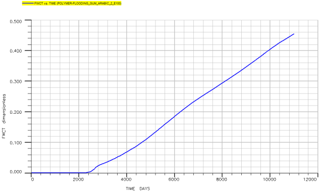
Figure 16. Field Water Cut (FWCT) against Time (days) for Polymer Concentration (0.3% wt.).

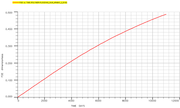
In figure 15, polymer concentration of 0.3wt% was injected which gave an oil recovery of 44.3%. The increase in oil recovery using polymer flooding is the fact that polymer increases the viscosity of the injected fluid (water) which helped to push the oil to the production well, hence, enhancing oil recovery. It is also important to note that, polymer aided in reservoir sweep efficiency via mobility control of injected water. Figure 16 indicate that water production started in one thousand, eight hundred days which means that more oil was produced from this well before water breakthrough and field water cut was 50.0%.

Download: Download full-size image

Figure 17. Field Oil Efficiency (oil recovery) against Time (days) for Polymer Concentration (0.4% wt.).

Download: Download full-size image

Figure 18. Field Water Cut (FWCT) against time (days) for Polymer Concentration (0.4% wt.).

Polymer flooding of 0.4wt% showed an increase in oil recovery of 48.4% (figure 17). The result suggest that concentration has a significant effect on oil recovery in polymer flooding. As more polymer was injected into the reservoir, more oil was recovered. In addition, figure 18, showed water-cut of 45.0% and water breakthrough time started at two thousand, three hundred days of polymer injection.

Download: Download full-size image

Figure 19. Field Oil Efficiency (oil recovery) against Time (days) for Polymer Concentration (0.5% wt.).

Download: Download full-size image

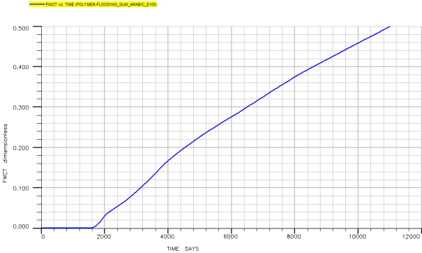
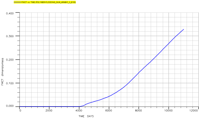
Figure 20. Field Water Cut (FWCT) against Time (days) for Polymer Concentration (0.5% wt.).

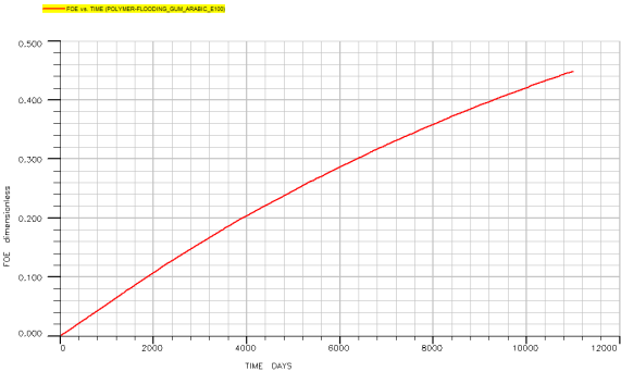
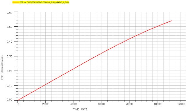
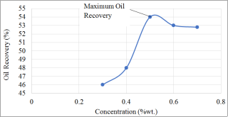
In figure 19, there was appreciably increase in oil recovery of 54.0% at polymer flooding of 0.5%wt. Increase in the concentration of polymer injection has a great effect in oil production. Polymer flooding had the highest oil recovery from the 80% oil in place in the reservoir. The results clearly suggest that polymer flooding have a greater sweep efficiency of oil when compared to water and surfactant flooding. Field water cut reduced to 33.0%. This means that oil was produced for four thousand days before water breakthrough as showed in figure 20. However, more surfactant and polymer at concentration of 0.6%wt. and 0.7%wt. was injected into the reservoir which oil recovery did not increase further. Hence, increase in oil recovery stopped at concentration of 0.5%wt.

Download: Download full-size image

Figure 21. Oil Recovery against Polymer Flooding Concentration.

Download: Download full-size image

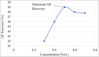
Figure 22. Oil Recovery against Surfactant Flooding Concentration.

Figures 21 and 22 indicates the maximum oil recovery for the surfactant-polymer flooding. The graphs showed that oil recovery was highest at concentration of 0.5%wt. At the concentration of 0.6%wt. and 0.7%wt. of surfactant and polymer injection, oil recovery did not increase further.

7. Conclusions

The study modeled 3-D reservoir using Eclipse software. Diffusivity equation of the simulated reservoir was derived which governed the fluid flow in a porous media to obtain the pressure distribution of the reservoir. The diffusivity equation was solved using Python codes (Jupyter Library). Simulation was carried out using surfactant-polymer to evaluate its performance in enhanced oil recovery. The following conclusions was drawn from the simulation study;

1) The implicit formulation results showed that reservoir pressure increases with time as oil production continued and water saturation decreases for the reservoir grid blocks.

2) Waterflooding had oil recovery of 38.0%, surfactant flooding had oil recoveries of 42.0%, 46.0%, and 49.0% while polymer flooding had oil recoveries of 46.0%, 48.0% and 54.0% respectively.

3) Reservoir water-cut was very high during waterflooding (59.0%) which indicates early water breakthrough time. However, polymer flooding had low water-cut of (33.0%) at 0.5%wt. concentration and delayed water breakthrough time was observed at 4000 days.

Acknowledgments

The authors wish to thank the Management of Abubakar Tafawa Balewa University for providing the laboratory space to carry out this research work. Special thanks go to Petroleum Technology Development Fund (PTDF) for the scholarship awarded to the first author.

Conflicts of Interest

The authors declared no conflict of interest.

References

[1]	Abbas M. & Olafuyi O. (2015). Application of Cubic Spline Numerical Modelling on Displacement Mechanism. Petroleum & Coal 57(3) pp 225-233.
[2]	Agi A., Radzuan J., Jeffrey G., & Onyekonwu M. (2018). Natural Polymer Flow Behavior in Porous Media for Enhanced Oil Recovery Applications: A Review. Journal of Petroleum Exploration and Production Technology. 8: pp 1349–1362.
[3]	Akpan E. A., Ogolo O., Ogiriki S., Aminu Y. K. & Daniel A., (2019). Numerical Simulation of Enhanced Oil Recovery Using Gum Arabic Polymer. Petroleum and Coal. 61(4) pp 660-671.
[4]	Bao K., Lie A., Mayner, O. & Liu, M. (2017). Fully Implicit Simulation of Polymer Flooding with MRST. Computational Geosciences. (10), pp 20-35.
[5]	Datta-Gupta A., Pope G. A., Sepehrnoori, K. & Thrasher R. L. (2018). A Symmetric, Positive Definite Formulation of a Three-Dimensional Micellar/Polymer Simulator. SPE Reservoir Engineering, vol. 1, no. 6, pp. 622-632.
[6]	Dogru, A. H., Mitsuishi, H. & Yamamoto, R. H. (2019). Numerical Simulation of Micellar Polymer Field Processes, In: SPE Paper 13121, SPE Annual Technical Conference, Houston, Texas.
[7]	Ertekin, T., Abou-Kassem, J. H., & King, G. R. (2007). Basic Applied Reservoir Simulation, Society of Petroleum Engineers Textbook Series, Volume 10, Richardson, Texas, USA.
[8]	Izuwa N. C., Ihekoronye K. K., Obah B. O., & Nnakaihe S. E. (2019). Evaluation of Low Salinity Polymer Flooding in the Niger Delta Oil Fields. Journal of Advanced Research in Petroleum Technology & Management, Volume 5, Issue 3, Pp. No. 17-38.
[9]	Izuwa N. C., Nwogu N. C., Williams C. C., Ihekoronye K. K., Okereke N. U. & Onyejekwe M. I. (2021). Experimental Investigation of Impact of Low Salinity Surfactant Flooding for Enhance Oil Recovery: Niger Delta Field Application. Journal of Petroleum and Gas Engineering. Vol. 12 (2), pp. 55-64.
[10]	Onyekonwu M. O. & Sunmonu R. M. (2017). Enhanced Oil Recovery using Foam/Polymer Injection; A Mechanistic Approach. SPE 167589. Presented at the Nigeria Annual International Conference and Exhibition held in Lagos, Nigeria.
[11]	Pope, G. A. & Nelson, R. C. (2018). A Chemical Flooding Compositional Simulator, SPE Journal, vol. 18, no. 5, pp. 339-354.
[12]	Sowunmi, A., Vincent E. E., Orodu O. D., Oluwasanmi O., & Oputa A. (2022). Comparative Study of Biopolymer Flooding: A Core Flooding and Numerical Reservoir Simulator Validation Analysis. Hindawi Modelling and Simulation in Engineering, Volume 2, pp 1-12.
[13]	Scott, T., Sharpe, S. R., Sorbie, K. S., Clifford, P. J., Roberts, L. J., & Oakes, J. A. (2017). A General-Purpose Chemical Flood Simulator”, SPE Paper 16029, In: Symposium on Reservoir Simulation, San Antonio, Texas.
[14]	Todd, M. R. & Chase, C. A. (2016). A Numerical Simulator for Predicting Chemical Flood Performance, In: SPE Paper 7689, Reservoir Simulation Symposium, pp 1-10.

Cite This Article

Plain Text BibTeX RIS

APA Style

Kelechi, I. K., Zwalatha, M. R., Ibrahim, C. A., Hussein, M. (2024). Modelling and Simulation of a 3-D Reservoir for Enhanced Oil Recovery of ‘X’ Field in the Niger Delta Using Eclipse Software. American Journal of Mathematical and Computer Modelling, 9(3), 54-67. https://doi.org/10.11648/j.ajmcm.20240903.11

Copy | Download

ACS Style

Kelechi, I. K.; Zwalatha, M. R.; Ibrahim, C. A.; Hussein, M. Modelling and Simulation of a 3-D Reservoir for Enhanced Oil Recovery of ‘X’ Field in the Niger Delta Using Eclipse Software. Am. J. Math. Comput. Model. 2024, 9(3), 54-67. doi: 10.11648/j.ajmcm.20240903.11

Copy | Download

AMA Style

Kelechi IK, Zwalatha MR, Ibrahim CA, Hussein M. Modelling and Simulation of a 3-D Reservoir for Enhanced Oil Recovery of ‘X’ Field in the Niger Delta Using Eclipse Software. Am J Math Comput Model. 2024;9(3):54-67. doi: 10.11648/j.ajmcm.20240903.11

Copy | Download

@article{10.11648/j.ajmcm.20240903.11,
  author = {Ihekoronye Kingsley Kelechi and Milton Roy Zwalatha and Caleb Abdullahi Ibrahim and Mohammed Hussein},
  title = {Modelling and Simulation of a 3-D Reservoir for Enhanced Oil Recovery of ‘X’ Field in the Niger Delta Using Eclipse Software},
  journal = {American Journal of Mathematical and Computer Modelling},
  volume = {9},
  number = {3},
  pages = {54-67},
  doi = {10.11648/j.ajmcm.20240903.11},
  url = {https://doi.org/10.11648/j.ajmcm.20240903.11},
  eprint = {https://article.sciencepublishinggroup.com/pdf/10.11648.j.ajmcm.20240903.11},
  abstract = {Surfactant-polymer flooding is a tertiary enhanced oil recovery method used to recover oil that remained in the reservoir after the primary and secondary oil recovery mechanisms. Predicting the pressure in the reservoir is important for oil production as pressure changes with time. A suitable approach to achieve this task is to derive fluid flow equation based on the reservoir characteristics and solve them numerically which provide the solution to the mathematical fluid flow model (diffusivity equation). In this study, 3-D reservoir was modelled using Eclipse software. The fluid flow equations in a porous media were derived based on the simulated model and the reservoir conditions. Numerical solution using implicit formulation to solve the mathematical fluid flow model (diffusivity equation) was investigated by developing Python codes using Jupyter library to ascertain the pressure distribution for the reservoir and imported into Eclipse simulator. Simulation was carried out using surfactant-polymer and reservoir properties to determine the oil recovery. The results of the study showed that pressure increases with time as oil production continued, and water saturation decreased for the grid-cells of the reservoir. Waterflooding had oil recovery of 38.0% and water-cut of 59.0%, while surfactant flooding had oil recoveries of 42.0%, 46.5%, 49.0% and water-cut of 57.0%, 51.0%, 46.3%. In addition, polymer flooding had oil recoveries of 44.3%, 48.4%, 54.0% and water-cut of 50.0%, 45.0% and 33.0% respectively at different concentrations of 0.3%wt. 0.4%wt. and 0.5%wt.
},
 year = {2024}
}

Copy | Download

TY - JOUR
T1 - Modelling and Simulation of a 3-D Reservoir for Enhanced Oil Recovery of ‘X’ Field in the Niger Delta Using Eclipse Software
AU - Ihekoronye Kingsley Kelechi
AU - Milton Roy Zwalatha
AU - Caleb Abdullahi Ibrahim
AU - Mohammed Hussein
Y1 - 2024/08/30
PY - 2024
N1 - https://doi.org/10.11648/j.ajmcm.20240903.11
DO - 10.11648/j.ajmcm.20240903.11
T2 - American Journal of Mathematical and Computer Modelling
JF - American Journal of Mathematical and Computer Modelling
JO - American Journal of Mathematical and Computer Modelling
SP - 54
EP - 67
PB - Science Publishing Group
SN - 2578-8280
UR - https://doi.org/10.11648/j.ajmcm.20240903.11
AB - Surfactant-polymer flooding is a tertiary enhanced oil recovery method used to recover oil that remained in the reservoir after the primary and secondary oil recovery mechanisms. Predicting the pressure in the reservoir is important for oil production as pressure changes with time. A suitable approach to achieve this task is to derive fluid flow equation based on the reservoir characteristics and solve them numerically which provide the solution to the mathematical fluid flow model (diffusivity equation). In this study, 3-D reservoir was modelled using Eclipse software. The fluid flow equations in a porous media were derived based on the simulated model and the reservoir conditions. Numerical solution using implicit formulation to solve the mathematical fluid flow model (diffusivity equation) was investigated by developing Python codes using Jupyter library to ascertain the pressure distribution for the reservoir and imported into Eclipse simulator. Simulation was carried out using surfactant-polymer and reservoir properties to determine the oil recovery. The results of the study showed that pressure increases with time as oil production continued, and water saturation decreased for the grid-cells of the reservoir. Waterflooding had oil recovery of 38.0% and water-cut of 59.0%, while surfactant flooding had oil recoveries of 42.0%, 46.5%, 49.0% and water-cut of 57.0%, 51.0%, 46.3%. In addition, polymer flooding had oil recoveries of 44.3%, 48.4%, 54.0% and water-cut of 50.0%, 45.0% and 33.0% respectively at different concentrations of 0.3%wt. 0.4%wt. and 0.5%wt.

VL - 9
IS - 3
ER -

Copy | Download

Author Information

Ihekoronye Kingsley Kelechi

Department of Petroleum Engineering, Abubakar Tafawa Balewa University (ATBU), Bauchi, Nigeria

Contact Email

http://orcid.org/0000-0001-6602-2593
Milton Roy Zwalatha

Department of Petroleum Engineering, Abubakar Tafawa Balewa University (ATBU), Bauchi, Nigeria

Contact Email
Caleb Abdullahi Ibrahim

Department of Petroleum Engineering, Abubakar Tafawa Balewa University (ATBU), Bauchi, Nigeria

Contact Email
Mohammed Hussein

Department of Petroleum Engineering, Federal University of Technology Owerri, Nigeria

Contact Email

Download PDF

Table 1

Table 1. Reservoir Rock and Fluid Properties.

Plain Text BibTeX RIS

APA Style

Kelechi, I. K., Zwalatha, M. R., Ibrahim, C. A., Hussein, M. (2024). Modelling and Simulation of a 3-D Reservoir for Enhanced Oil Recovery of ‘X’ Field in the Niger Delta Using Eclipse Software. American Journal of Mathematical and Computer Modelling, 9(3), 54-67. https://doi.org/10.11648/j.ajmcm.20240903.11

Copy | Download

ACS Style

Kelechi, I. K.; Zwalatha, M. R.; Ibrahim, C. A.; Hussein, M. Modelling and Simulation of a 3-D Reservoir for Enhanced Oil Recovery of ‘X’ Field in the Niger Delta Using Eclipse Software. Am. J. Math. Comput. Model. 2024, 9(3), 54-67. doi: 10.11648/j.ajmcm.20240903.11

Copy | Download

AMA Style

Kelechi IK, Zwalatha MR, Ibrahim CA, Hussein M. Modelling and Simulation of a 3-D Reservoir for Enhanced Oil Recovery of ‘X’ Field in the Niger Delta Using Eclipse Software. Am J Math Comput Model. 2024;9(3):54-67. doi: 10.11648/j.ajmcm.20240903.11

Copy | Download

@article{10.11648/j.ajmcm.20240903.11,
  author = {Ihekoronye Kingsley Kelechi and Milton Roy Zwalatha and Caleb Abdullahi Ibrahim and Mohammed Hussein},
  title = {Modelling and Simulation of a 3-D Reservoir for Enhanced Oil Recovery of ‘X’ Field in the Niger Delta Using Eclipse Software},
  journal = {American Journal of Mathematical and Computer Modelling},
  volume = {9},
  number = {3},
  pages = {54-67},
  doi = {10.11648/j.ajmcm.20240903.11},
  url = {https://doi.org/10.11648/j.ajmcm.20240903.11},
  eprint = {https://article.sciencepublishinggroup.com/pdf/10.11648.j.ajmcm.20240903.11},
  abstract = {Surfactant-polymer flooding is a tertiary enhanced oil recovery method used to recover oil that remained in the reservoir after the primary and secondary oil recovery mechanisms. Predicting the pressure in the reservoir is important for oil production as pressure changes with time. A suitable approach to achieve this task is to derive fluid flow equation based on the reservoir characteristics and solve them numerically which provide the solution to the mathematical fluid flow model (diffusivity equation). In this study, 3-D reservoir was modelled using Eclipse software. The fluid flow equations in a porous media were derived based on the simulated model and the reservoir conditions. Numerical solution using implicit formulation to solve the mathematical fluid flow model (diffusivity equation) was investigated by developing Python codes using Jupyter library to ascertain the pressure distribution for the reservoir and imported into Eclipse simulator. Simulation was carried out using surfactant-polymer and reservoir properties to determine the oil recovery. The results of the study showed that pressure increases with time as oil production continued, and water saturation decreased for the grid-cells of the reservoir. Waterflooding had oil recovery of 38.0% and water-cut of 59.0%, while surfactant flooding had oil recoveries of 42.0%, 46.5%, 49.0% and water-cut of 57.0%, 51.0%, 46.3%. In addition, polymer flooding had oil recoveries of 44.3%, 48.4%, 54.0% and water-cut of 50.0%, 45.0% and 33.0% respectively at different concentrations of 0.3%wt. 0.4%wt. and 0.5%wt.
},
 year = {2024}
}

Copy | Download

VL - 9
IS - 3
ER -

Copy | Download