A Band Spectral Density Regression of Exports on the Gross Domestic Product of the Kenyan Economy

Safari Godfrey Lyece; Joseph Kyalo Mung’atu; Jane Aduda Akinyi

doi:doi:10.11648/j.ajtas.20251401.13

Research Article |

| Peer-Reviewed

A Band Spectral Density Regression of Exports on the Gross Domestic Product of the Kenyan Economy

Safari Godfrey Lyece^*, Joseph Kyalo Mung’atu, Jane Aduda Akinyi

Published in American Journal of Theoretical and Applied Statistics (Volume 14, Issue 1)

Received: 16 October 2023 Accepted: 13 November 2024 Published: 10 February 2025

Views: Downloads:

Download PDF

Share This Article

Twitter
Linked In
Facebook

Abstract

The aim of this study is to be able to find the relationship between two time series variables applying the spectral analysis techniques. The spectral analysis techniques would enable the study explain this relationship in a more advanced way particularly in the frequency domain. Since the study will be focusing on two time series, we shall use the cross spectral density function which shall be estimated based on the cross periodogram function. The Cross spectral density function would give the power distribution of the two times series across the frequency domain. In this case each power will be associated with a frequency. Then we shall apply the square coherence function to find whether there is any association or the presence of a seasonality effect between the two series signals at each frequency. This would help us determine whether these two series are dependent or independent. Once the association has been established, we shall apply the Frequency Response Function (FRF) to estimate the effect the input variable in this case the independent variable has on the output in this case the dependent variable across the frequency domain. Finally, the study would use an F Test to determine which of the input frequencies are significant in explaining the output or the output variable.

Published in	American Journal of Theoretical and Applied Statistics (Volume 14, Issue 1)
DOI	10.11648/j.ajtas.20251401.13
Page(s)	30-37
Creative Commons	This is an Open Access article, distributed under the terms of the Creative Commons Attribution 4.0 International License (http://creativecommons.org/licenses/by/4.0/), which permits unrestricted use, distribution and reproduction in any medium or format, provided the original work is properly cited.
Copyright	Copyright © The Author(s), 2025. Published by Science Publishing Group

Keywords

Spectral Analysis Techniques, Squared Coherency, Frequency Response, Function, Cross-Spectral Density Function, Bandwidth

1. Introduction

For many years agricultural products have been central to Kenya’s exports industry with tea and horticulture being the most fundamental exports. Other commodities that have been found in the export sector include coffee, tobacco, textiles, petroleum products, cement, iron and steel.

An economic prospect, say above 6% Gross Domestic Product (GDP) growth as a result of expansion in telecommunications, constructions, transport and recovery in the agricultural sector attributed to improvements supported by a pool of English-speaking professional workers and a higher level of computing literacy skills among the young people. The question is how much of this growth would be attributed to exports in the country?

This study will try to establish the significant effect the exports have on the overall economic growth of the Republic of Kenya which is determined by the Gross Domestic Product (GDP) using the times series model known as the spectral density regression. For years Kenya has been exporting a number of goods and services to her neighbours, other African countries and other parts of different continents including the United Kingdom, United States of America, Netherlands, India and France. The number of exports has significantly increased attributable to advancement of technology which has enabled Kenya to focus on the addition of value to its exports, improvement of road infrastructure in the rural areas. This has enabled perishable goods access the international market within the shortest time possible.

This study aims at finding the contribution of exports to overall economic growth of the Republic of Kenya from the year 2009-2020. We will take our frequency ω as quarterly which will imply, we are going to have a total of 42 quarter years for the entire period of the analysis. According to the World Bank reports (2014) the Kenyan Economy measured by the (GDP) was worth 60.94 billion US Dollars. But it fails to break these findings into different horizon to reflect how different components of exports had an impact to this development. Therefore, with the Band Spectral Density Regression (BSDR) being the modification of the classical linear regression, will enable us look at the contribution of exports to the movement of the Kenyan Gross Domestic Product (GDP) in the perspective of different frequency components.

The specific objectives for this study are: To estimate the cross-spectrum density function of the Kenyan GDP and Exports which will enable us to estimate the Squared Coherency of the Kenyan GDP and Exports. When the Squared Coherency has been found we shall apply the Frequency Response function to describe the linear relationship between the two variables in the frequency domain. Finally, we shall determine which exports variable frequencies are significant to the contribution of the GDP variable.

The study is effective for policy making. It would enable us know the contribution the principle exports have on the depended variable GDP at the market price in the frequency domain. For example, the method of cross spectral density analysis would show how the power of the two times series signals are distributed across the frequency domain. The frequencies with/without similar seasonal components would be identified through the use of the Squared coherence function which would suggest whether or not the two times series are correlated or uncorrelated. In the event that the two series are found to be correlated, then the study would estimate the contribution exports have on the GDP through the application of Frequency Response Function FRF. Once the FRF has been estimated, the study would identify the significant exports frequencies that are fundamental in the GDP contribution. The significant frequencies would indicate the times in quarters this contribution to the GDP happens. This would enable policy makers aim at maximizing the production of exports while improving quality at this particular time when exports contribution to the GDP is significant.

Literature Review

Spectral density regression Analysis has a very long history in the field of Econometrics according to (Chartfield, 2004)

[1]

. Its application ranging from Economic/business cycle analysis to the evaluation of prices and Option according to (Ibrahim, 2014)

[2]

This Kind of analysis relies very much on transforming the times series data into a fourier transform as observed by (Croux, 2001)

[3]

. However, according to (Ramsey, 2002)

[4]

wavelets transform have also been applied to study times series data in both time and frequency domain. In this study cross-spectral density function (CSDF) which is calculated using fourier transform as shown by (Oppenheim, 2001)

[5]

shall form the basis of our spectral density regression.

Alot of analytical studies about the relationship between export and Gross domestic product growth (GDP) has been done by many scholars particularly in the Emerging Economies. For example, (Jung, 1985)

[6]

examined the casuality between economic growth and exports for thirty seven (37) emarging economies and found evidence that support export-led Growth hypothesis for Indonesia, Ecuador, Egypt and Costa Rica from the period of 1950 to 1981. (Chow, 1987)

[7]

applied Sim’s casuality in a bivariate model to investigate casuality between industrial output and exports of industrial goods in eight (8) Newly Industrial Countries (NIC).

In the India context, several emperical studies have been conducted. (Dhawan, 1999)

[8]

also examined the Export led Growth hypothesis by investigating the association between exports, terms of trade and the real Gross Domestic Product (GDP) for India from 1969 to 1993 applying the Vector Autoregressive (VAR) model. In this study they brought in a multivariate approach using the Johansen’s Co-integration technique. They were able to find a long-run relationship between these variables and also casual association which flowed from the terms of trade to the growth of exports which boasted the growth of the (GDP). They however concluded that the casual relationship between the Gross Domestic Product (GDP) and exports seems to be a short-run phenomenon.

Many dynamics systems ranging from geographical systems (Marinho, 2013)

[9]

and (Campillo M.)

[10]

through brain networks (Achard S., 2008)

[11]

and (Ciuciu, 2014)

[12]

or metrological data by (Vassoler. R. T., 2012)

[13]

have been shown to express scale-free correlation both in the univariate dynamics of their individual constituents as well as in their interaction. In both scenarios power law relationship can be established between correlation and the scale of the observation according to (Podobnik, 2008)

[14].

In the Health context (Lu W. L., 2021)

[15]

applied the spectral methods to analyze the effect of respiration on the heart rate. The analysis was carried out on fourty two healthy individuals where the cross spectral analysis of electrocardigraphic (ECG) and nostril airflow signals was carried out to investigate the effect of respiration on the heart rate.

The results were compared with the convectional Heart Rate Variability (HRV) measures. It was found that there was a peak at around 0.3 HZ in the Cross-spectrum of (ECG) and the nostril airflow. The Cross- Spectral normalized high frequency power (nHFPcs) was significantly larger than that of the Conventional HRV while the crossspectral normalized very low frequency power (nVLFPcs), normalized low frequency power (nLFPcs), and normalized low-/high frequency power ratio (LHRcs) were significantly lower than the conventional (HRV). There was a positive correlation between the cross spectral (nLFPcs) and (LHRcs) with their corresponding Conventional HRV measure. The study concludes that cross-spectral analysis of (ECG) and nostril airflow signals identifies two respiratory frequencies at around 0.3 Hz and can yield significantly enhanced (nHFPcs) and significantly suppressed (nVLFPcs), as compared to their counterparts in conventional (HRV). Both very low-frequency and high-frequency components of (HRV) are caused in part or mainly by respiration.

(Ameera, 2019)

[16]

applied the power spectral density function to analyze the brain signals features between pleasure and displeasure mental states. In this study brainwaves were divided into five sub-frequency bands namely alpha (8-13 HZ), beta (13-30 HZ), gamma (30-100 HZ), theta (4-8 HZ), delta (1-4 HZ). The alpha and beta waves were analyzed to investigate the mental states. The alpha waves were found to be the most potential to be used in order to differentiate between pleasure and displeasure features.

(Manjarrez, 2024-03)

[17]

employed the Fast Fourier to calculate the power spectral density (PSD) of COVID-19 mortality waves from January 22, 2020 to March 9, 2023 in 199 countries. Two dominant peaks were identified in the grand average (PSD). One at a frequency of 1.15 waves per year (i.e. one in every 10.4 months) and another at 2.7 waves per year (i.e. one in every 4.4 months).

2. Methods

In this study we have two times series which we aim to establish their linear relationship in the frequency domain applying the spectral analysis methods. The effect of the exports on the Gross Domestic product would be examined across all the frequencies from the year 2009-2020 where observations will be made quarterly during this period.

2.1. Cross-Spectrum of Two Times Series

The cross-spectrum of a bivariate process is measured at a unit interval of time as the Fourier transformation of the cross-covariance function γ(t, k) is given as

f_{xy} (ω) = \frac{1}{π} Σ γ_{xy} (k) \exp - iω

where

ω

is frequency in quarters

γ_{xy} (k) = cov (x_{t}, y_{t + k})

for

0 < ω < π

2.2. Estimation of the Cross Spectrum Function

Spectral analysis is a term that used to estimate the cross-spectrum over the the whole range of frequencies of two times series. There are many techniques that can be used in spectral analysis. These include smoothing of cross-periodogram, Trancating the cross-covariance function using Fourier transform on truncated cross-covariance weights, Hanning, Hamming, and the fast Fourier transform. In this project we would estimate the cross-spectrum with the aid of the smoothing of the periodogram. This is because periodogram in itself is an asymptotically unbiased but not a consistent estimator of the cross-spectrum from the fact that the variance does not decrease as the number of times series observations increase.

2.3. Smoothing the Cross-Periodogram

Since the cross-periodogram is asymptotically unbiased but not a consistent estimator of the true cross-spectrum, we would be required to divide the cross-spectrum into 2m+1 ordinates and take the average. The smoothed cross-spectrum would be given as

f_{xy} (ω) = \frac{1}{2 m + 1} \sum f_{xy} (ω)

where is

\frac{1}{2 m + 1}

Daniell spectral window which we shall denote as w_m(k) named after P. J. Daniell who first used it in 1940s.

Now, the choice of m should be made so that there is a trade-off between reducing variability and introducing bias. This is because too large value of m would reduce variability and introduce bias resulting to loss of some important information in the smoothed cross-spectrum whereas reducing the value of m would increase variability and reduce the bias. Therefore, we can determine the value of m through a trial-and-error approach put in mind the trade-off between reducing variability at the expense of introduction of bias. We shall try three different values of m. The small value of m would give as an idea of where the large peaks in the cross spectrum are and can be large in number which are spurious while the large value of m would produce curves that are too smooth. Therefore, a compromise may be found with a third value of m.

The choice of m should be based on the number of times series observations n. Chat-field (2004) suggested using

m = \sqrt{n}

as a compromise value,

m = \frac{1}{2} \sqrt{n}

as the small value, and

m = 2 \sqrt n

as the highest value to be used in the Daniell spectral window.

2.4. Squared Coherency of Two Times Series

The Square Coherency measures the relationship between these two times series will be interpreted as the square correlation coefficient between the spectral density function of our output in this case the Kenyan GDP at the market price and the spectral density function of our input which in this case is the Principal Exports also at the market prices calculated at each frequency ω_j.

h_{xy}^{2} (ω) = {(c}^{2} (ω) + q^{2} (ω)) / f_{x} (w) f_{y} (w)

which is equivalent to

h_{xy}^{2} (ω_{j}) = \frac{α_{xy}^{2} (ω_{j})}{f_{x} (ω_{j}) f_{y} (ω_{j})}

where

ω_{j} = \frac{π_{j}}{N}

for

j = 0, 1, 2, 3, \dots, \frac{N}{2}

The estimated square coherancy will be between 0 and 1 where a value close to zero indicates the two stationary times series are uncorrelated while a value close to one indicates that the two stationary series are related at frequency ω.

2.5. Response Function of a Times Series as a Result of Another Times Series

Suppose we have quarterly observations on exports and GDP from 2009-2020 and we wish to use these observations to estimate the frequency response function of a linear system. The frequency response function shall be denoted as H(ω). The frequency response function to be estimated describes this particular linear system in the frequency domain which will be estimated from the estimated cross-spectrum of both the input and the output variables in the system.

f_{xy} = H (ω) f_{x} (ω)

for 0

< ω < π

which is equivalent to

H (ω_{j}) = \frac{f_{xy} (ω_{j})}{N}

where

ω_{j} = \frac{π_{j}}{2}

for

j = 0, 1, 2, 3, 4, \dots, N

2.6. Determination of Impactful Frequencies of Principle Exports to the Kenyan GDP

Analysing times series processes in the frequency domain would enable us to discover which frequencies dominate in the signal’s energy distribution as presented by the cross-spectral density function of the two times series signals. Therefore, in our study the frequency dominance would help us identify which particular principle export frequencies are fundamental in the contribution of the Kenyan GDP at the market prices. This frequency contribution of the Principle Exports to the Kenyan GDP would be easily identified from the Frequency Response Function (FRF). The FRF gives the gain information better known as regression coefficient as a function of frequencies. We shall use the F −test statistic to identify the particular Principle Exports frequencies with coeffients which are significant in the contribution to the Kenyan GDP. Our significance level α would be 5% and the F −test would be distributed with 2 and 2m−2 degrees of freedom where m in this case is based on the spectral window used in smoothing the cross periodiogram.

So the lower 5% level would be

F_{2, 2 m - 2 (α = 0.025)}

while the upper 95% level would be

F_{2, 2 m - 2 (α = 0.975)}

Download: Download full-size image

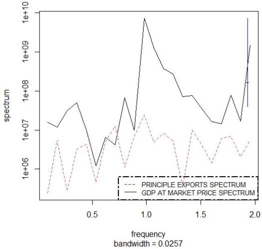
Figure 1. The raw cross Spectral Density Relationship between GDP at Market Prices and the Principle Exports.

Now that we have the two times series with the trend component removed, we can now use the periodgram to get the sample estimate of the population function called the cross spectral density which is the frequency domain characterization of the stationary series. From Figure 1 the cross-periodogram relationship between the two times series isn’t well described because of too much variability observed. Even though the peak from the above raw cross-periodigram can be spotted, it cannot be considered to be a true peak because of its spurious in nature which is attributed to the raw crossperiodigram lack of trade off between the variance and the bias. To reduce the variability we need to average the 2m+1 values of the cross-periodogram over a small interval of frequencies. We need to smooth the cross-periodigram or the sampled cross-spectral density function using the spectral windows known as Daniel Window. The choice of m should be made so that there is a trade-off between reducing variability and introducing bias. We can determine the value of m through a trial-and-error approach keeping in mind the trade-off between reducing variability at the expense of introduction of bias. We shall try three different values of m. The small value of m would give us an idea of where the large peaks in the cross spectrum are and can be large in number which are spurious while the large value of m would produce curves that are too smooth. Therefore, a compromise may be found with a third value of m. The choice of m should be based on the number of times series observations n. Taking the value of m_s= 3 as the value of our spectral window in smoothing the raw cross-periodgram, we obtain the graph shown below.

Exports with spectral window m = 3

Download: Download full-size image

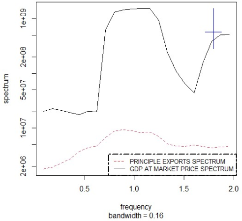
Figure 2. Smoothed cross Spectrum Function of GDP at Market Price and Principle.

When the spectral window used to smooth the cross-periodogram is m = 13, we obtain Figure 3. From Figure 3, the estimated spectrum has been over smoothed which.

Download: Download full-size image

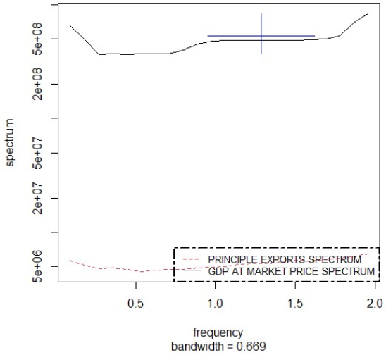
Figure 3. Smoothed cross Spectrum Function of GDP at Market Price and Principle Exports with spectral window m_l= 13.

Has resulted in difficulty in identify the peak. Again, the bandwidth is very large as shown by the horizontal line in the +. This is also an indication that the trade off between reducing variability and introducing bias has not been achieved.

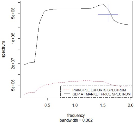
Therefore, with already determined compromised value of m_c= 7 we can now have the spectrum relationship of the two times series in the frequency domain as shown in the figure below. The crosshair displayed in the right-hand corner gives us the 95% confidence interval and the bandwidth used in the cross-spectrum density estimation. Here, the vertical length is the length (width) of the confidence interval, while the horizontal line indicates the central point of the confidence interval and the width (length) of the horizontal segment matches the bandwidth of the spectral window.

Exports with spectral window m_c= 7

Download: Download full-size image

Figure 4. Smoothed Cross Spectrum Function of GDP at Market Price and Principle.

From Figure 3 the energy distribution of the two times series signals is well presented and one can be able to note the areas with high energy concentration known as the peak as well as areas with low energy concentration known as the trough.

From the results for our first objective after applying non-parametric methods to estimate the cross-spectrum function, we have found that both the principle exports and the GDP at the market prices all measured in million dollars, on average have their peak at the frequency ω = 0.25*1.5111111= 0.3778. This implies that on average the principle exports have their highest contribution to the Kenyan GDP on every

\frac{1}{3.778} ≃ 2.65

_.quarter. The same variables have their trough at the frequency ω = 0.25*0.0888889=0.022222225. This implies that on average the Principle exports have very low contribution to the Kenyan GDP on

\frac{1}{0.022222225} ≃ 45

quarter that is on every 45th quarter of the calender year.

Now, from the estimated cross spectrum we can obtain the squared Coherency between the GDP at the Market Price and the Principle Exports. The coherency estimates would determine the amount of relationship between the two series on each frequency. The Coherency estimates plot is shown in Figure 5.

Download: Download full-size image

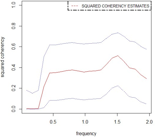
Figure 5. Squared Coherency Estimates of the GDP at Market Price and Principle Exports on Each Frequency.

The Square coherency which is a measure of degree of the dependency between two times series at a similar frequency component shows that this dependency between the Principle exports and GDP at the Market prices lies between 0.0006545702 and 0.5127675808 at frequency ω_j=0.25*0.177778'0.0444 and

ω j = 0.25 * 1.51111111 ≃ 0.3778

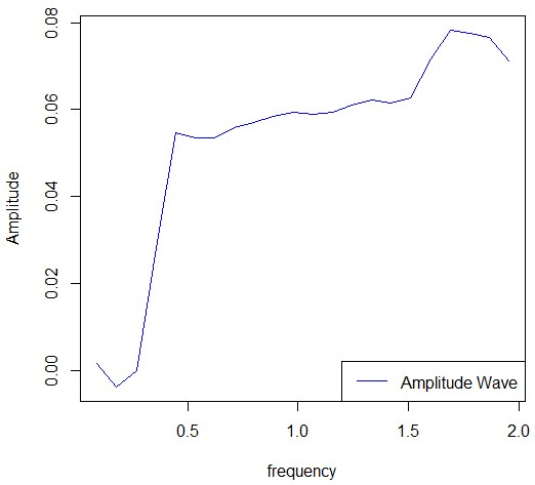
respectively. This is a strong indication that the two variables are not uncorrelated and therefore, this is an indication that a change in the Kenyan GDP can be attributed to a change of other variables one of them being the Principle Exports at the Market Prices. Having established some Square Coherency between our times series processes, we need to estimate the exact contribution that Principle Exports have to the Kenyan GDP across the frequency bands. From the frequency response function computation, we can see the gain as given by the amplitude increasing significantly across all the frequencies except at frequencies ω_j= 0.0444, ω_j= 0.06667. 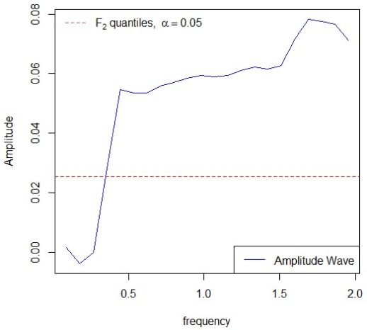From this case the highest gain that can be attributed by the Principle Exports to the GDP is roughly 0.078 at frequency ω_j= 0.4222 as shown in Figure 6 below. Finally, We identify which of the above Principle Exports frequencies are significant to the Kenyan GDP contribution. We used the F −Test to check for the significance that is whether the regression coeficients given by the amplitude are significant in explaining the contribution of the Principle Exports to the Kenyan GDP across the frequency band. Therefore, the 95% confidence interval is between F₂,₂₄(0.025) = 0.02534453 and F₂,₂₄(0.975) = 4.318726. From Figure 6. we find that the frequencies from ω_j= 0.25∗0.35555556 ≃0.089 onward that is the higher frequencies are significant in explaining the Kenyan GDP. This is because the corresponding amplitude which represents the Principle Exports coefficients from the frequency ω_j= 0.25∗0.35555556 ' 0.089 lies within the our confidence interval [0.02534453,4.318726] with the highest contribution to the Kenyan GDP being 0.078 corresponding to the frequency ω_j' 0.4222 which translates to the

\frac{1}{0.4222} ≃ 2.368 th

quarter. Therefore, it will be prudent to say that higher-frequency components are very important in explaining the Principle Exports and the Kenyan GDP relationship. That is high-frequency Principle exports components with periods less than

\frac{1}{0.089} ≃ 11.24

quarters are insignificant in explaining the Kenyan GDP at market prices.

Download: Download full-size image

Figure 6. The Estimated Frequency Response Function between the Input Principle Exports and the output Kenyan GDP at the Market Prices.

Download: Download full-size image

Figure 7. 95% Confidence band for the Frequency Response Function.

3. Conclusion

The study has shown that we can use spectral analysis techniques to study the effect a times series signal referred to as input has on another times series signal referred to as output in the frequency domain. The research has shown that Principle exports and the Kenyan GDP have varing components across all the frequencies which clearly indicates that these two variables are correlated. Therefore, we can comfortably state that GDP is a variable associated with other variables one of them being the Principle Exports at the Market Prices.

From the study, the Spectral Regression technique has enabled us learn that even in as much as we export a lot of agricultural products such as Tea, Coffee and Horticulture, even though their contribution to the Kenyan GDP is significant on higher frequencies particularly on periods less than 11.24 quarters, such contributions seem to be slightly small. For example, we find that from the higher frequency components band that the highest contribution of the Principle Exports to the Kenyan GDP is around 0.078 which is realized at frequency ω = 0.3778 which translates to the 2.65th quarter while the lowest contribution is around 0.001468 at frequency ω = 0.0222 which translates to the 45th quarter of the calendar year on the low frequency component band. I recommend that different method such as Hanning, Hamming, Trancating the cross covariance function using the Fourier transform on the trancated cross-covariance function to estimate the cross spectral density function should be applied in order to estimate the relationship between two times series in the frequency domain.

4. Recommendation

I recommend that more resources should be channelled to the export sector particularly the cash crop sector to increase the present yields. I also recommend further studies to be taken on the contribution of other variables such as Government Expenditures and Investments to the Kenyan GDP so that we can make a comparison with this study to ascertain which variable(s) has(have) the highest impact to the Kenyan GDP in the frequency domain.

Abbreviations

GDF	Gross Domestic Product
FRF	Frequency Response Function
HRV	Heart Rate Variability
NHFPcs	Normalized High Frequency Power
nLFPcs	Normalized Low Frequency Power
LHRcs	Normalized Low-/High Frequency Power Ratio
ECG	Electrocardigraphic
CSDF	Cross-spectral Density Function

Acknowledgments

I would like to thank Mr. Gregory Michael Mbishi for his great encouragement to undertake this impactful research which has established the contribution that Exports have on the overall Gross Domestic Product of Kenya. I would also like to thank my supervisors for their insightful comments which have yielded to a fruitful and impactful finding which when applied in decision making purpose would boast the growth of the Economy of Kenya. I would also like to thank the Central Bank of Kenya for providing us with the datasets which were used in the study.

Conflicts of Interest

The authors of this article do not have any conflict of interest.

References

[1]	Chartfield, C. (2004). The analysis of time series: an introduction. CRC Press, Florida, US.
[2]	Ibrahim, S. O. (2014). Pricing extendible options using the fast fourier transform. Mathematical Problems in Engineering.
[3]	Croux, C. F. (2001). A measure of comovement for economic variables: Theory and empirics. Review of Economics and Statistics, 83(2): 232-241.
[4]	Ramsey, J. B. (2002). Wavelets in economics and finance: Past and future. Studies in Nonlinear Dynamics and Econometrics, 6(3).
[5]	Oppenheim, A. V. (2001). Discrete-time Signal Processing. Vol 2. Upper Saddle River, NJ: Prentice Hall.
[6]	Jung, W. M. (1985). Exports, growth and causality in developing countries. Journal of development economics, 18(1): 1-12.
[7]	Chow, P. C. (1987). Causality between export growth and industrial development empirial evidence from the nics. Journal of development Economics, 55-63.
[8]	Dhawan, U. B. (1999). Re-examining export-led growth hypothesis: a multivariate cointegration analysis for India. Applied Economics, 31(4): 525-530.
[9]	Marinho, E. S. (2013). Using detrended cross-correlation analysis in geophyical data. Physical A: Statistical Mechanics and its Application, 2195-2201.
[10]	Campillo M., P. A. (n.d.). Long-range correlations in the diffuse seismic coda. Science.
[11]	Achard S., B. D.-L. (2008). Fractal connectivity of long-memory network. Physical Review E—Statistical, Nonlinear, and Soft Matter Physics, 036104.
[12]	Ciuciu, P. A. (2014). Interplay between functional connectivity and scale-free dynamics in intrinsic fMRI networks. Neuroimage, 248-263.
[13]	Vassoler. R. T., &. Z. (2012). DCCA cross- correlation coefficient apply in time series of air temperature and air relative humidity Physica A: Statistical Mechanics and its Applications. 2438-2443.
[14]	Podobnik, B. H. (2008). Modeling long-range cross-correlations in two-component ARFIMA and FIARCH processes. Physica A: Statistical Mechanics and its Applications. 3954-3959.
[15]	Lu, W. L. (2021). Cross-Spectral analysis of electrocardiographic and nostril airflow signals identifies two respiratory frequencies of heart rate modulation. Journal of Healthcare Engineering.
[16]	Ameera, A. A. (2019). Analysis of EEG Spectrumbands using power spectral density for pleasure and displeasure state. In IOP conference series Materials Science and engineering, 012030.
[17]	Manjarrez, E. D.-N. (2024-03). Power spectral density and similarity analysis of COVID-19 mortality waves across countries. medRxiv.

Cite This Article

Plain Text BibTeX RIS

APA Style

Lyece, S. G., Mung’atu, J. K., Akinyi, J. A. (2025). A Band Spectral Density Regression of Exports on the Gross Domestic Product of the Kenyan Economy. American Journal of Theoretical and Applied Statistics, 14(1), 30-37. https://doi.org/10.11648/j.ajtas.20251401.13

Copy | Download

ACS Style

Lyece, S. G.; Mung’atu, J. K.; Akinyi, J. A. A Band Spectral Density Regression of Exports on the Gross Domestic Product of the Kenyan Economy. Am. J. Theor. Appl. Stat. 2025, 14(1), 30-37. doi: 10.11648/j.ajtas.20251401.13

Copy | Download

AMA Style

Lyece SG, Mung’atu JK, Akinyi JA. A Band Spectral Density Regression of Exports on the Gross Domestic Product of the Kenyan Economy. Am J Theor Appl Stat. 2025;14(1):30-37. doi: 10.11648/j.ajtas.20251401.13

Copy | Download

@article{10.11648/j.ajtas.20251401.13,
  author = {Safari Godfrey Lyece and Joseph Kyalo Mung’atu and Jane Aduda Akinyi},
  title = {A Band Spectral Density Regression of Exports on the Gross Domestic Product of the Kenyan Economy
},
  journal = {American Journal of Theoretical and Applied Statistics},
  volume = {14},
  number = {1},
  pages = {30-37},
  doi = {10.11648/j.ajtas.20251401.13},
  url = {https://doi.org/10.11648/j.ajtas.20251401.13},
  eprint = {https://article.sciencepublishinggroup.com/pdf/10.11648.j.ajtas.20251401.13},
  abstract = {The aim of this study is to be able to find the relationship between two time series variables applying the spectral analysis techniques. The spectral analysis techniques would enable the study explain this relationship in a more advanced way particularly in the frequency domain. Since the study will be focusing on two time series, we shall use the cross spectral density function which shall be estimated based on the cross periodogram function. The Cross spectral density function would give the power distribution of the two times series across the frequency domain. In this case each power will be associated with a frequency. Then we shall apply the square coherence function to find whether there is any association or the presence of a seasonality effect between the two series signals at each frequency. This would help us determine whether these two series are dependent or independent. Once the association has been established, we shall apply the Frequency Response Function (FRF) to estimate the effect the input variable in this case the independent variable has on the output in this case the dependent variable across the frequency domain. Finally, the study would use an F Test to determine which of the input frequencies are significant in explaining the output or the output variable.
},
 year = {2025}
}

Copy | Download

TY  - JOUR
T1  - A Band Spectral Density Regression of Exports on the Gross Domestic Product of the Kenyan Economy

AU  - Safari Godfrey Lyece
AU  - Joseph Kyalo Mung’atu
AU  - Jane Aduda Akinyi
Y1  - 2025/02/10
PY  - 2025
N1  - https://doi.org/10.11648/j.ajtas.20251401.13
DO  - 10.11648/j.ajtas.20251401.13
T2  - American Journal of Theoretical and Applied Statistics
JF  - American Journal of Theoretical and Applied Statistics
JO  - American Journal of Theoretical and Applied Statistics
SP  - 30
EP  - 37
PB  - Science Publishing Group
SN  - 2326-9006
UR  - https://doi.org/10.11648/j.ajtas.20251401.13
AB  - The aim of this study is to be able to find the relationship between two time series variables applying the spectral analysis techniques. The spectral analysis techniques would enable the study explain this relationship in a more advanced way particularly in the frequency domain. Since the study will be focusing on two time series, we shall use the cross spectral density function which shall be estimated based on the cross periodogram function. The Cross spectral density function would give the power distribution of the two times series across the frequency domain. In this case each power will be associated with a frequency. Then we shall apply the square coherence function to find whether there is any association or the presence of a seasonality effect between the two series signals at each frequency. This would help us determine whether these two series are dependent or independent. Once the association has been established, we shall apply the Frequency Response Function (FRF) to estimate the effect the input variable in this case the independent variable has on the output in this case the dependent variable across the frequency domain. Finally, the study would use an F Test to determine which of the input frequencies are significant in explaining the output or the output variable.

VL  - 14
IS  - 1
ER  -

Copy | Download

Author Information

Safari Godfrey Lyece

Department of Statistics and Actuarial Sciences, Jomo Kenyatta University of Agriculture and Technology (JKUAT), Nairobi, Kenya

Contact Email
Joseph Kyalo Mung’atu

Department of Statistics and Actuarial Sciences, Jomo Kenyatta University of Agriculture and Technology (JKUAT), Nairobi, Kenya

Contact Email
Jane Aduda Akinyi

Department of Statistics and Actuarial Sciences, Jomo Kenyatta University of Agriculture and Technology (JKUAT), Nairobi, Kenya

Contact Email

Download PDF

Plain Text BibTeX RIS

APA Style

Lyece, S. G., Mung’atu, J. K., Akinyi, J. A. (2025). A Band Spectral Density Regression of Exports on the Gross Domestic Product of the Kenyan Economy. American Journal of Theoretical and Applied Statistics, 14(1), 30-37. https://doi.org/10.11648/j.ajtas.20251401.13

Copy | Download

ACS Style

Lyece, S. G.; Mung’atu, J. K.; Akinyi, J. A. A Band Spectral Density Regression of Exports on the Gross Domestic Product of the Kenyan Economy. Am. J. Theor. Appl. Stat. 2025, 14(1), 30-37. doi: 10.11648/j.ajtas.20251401.13

Copy | Download

AMA Style

Lyece SG, Mung’atu JK, Akinyi JA. A Band Spectral Density Regression of Exports on the Gross Domestic Product of the Kenyan Economy. Am J Theor Appl Stat. 2025;14(1):30-37. doi: 10.11648/j.ajtas.20251401.13

Copy | Download

@article{10.11648/j.ajtas.20251401.13,
  author = {Safari Godfrey Lyece and Joseph Kyalo Mung’atu and Jane Aduda Akinyi},
  title = {A Band Spectral Density Regression of Exports on the Gross Domestic Product of the Kenyan Economy
},
  journal = {American Journal of Theoretical and Applied Statistics},
  volume = {14},
  number = {1},
  pages = {30-37},
  doi = {10.11648/j.ajtas.20251401.13},
  url = {https://doi.org/10.11648/j.ajtas.20251401.13},
  eprint = {https://article.sciencepublishinggroup.com/pdf/10.11648.j.ajtas.20251401.13},
  abstract = {The aim of this study is to be able to find the relationship between two time series variables applying the spectral analysis techniques. The spectral analysis techniques would enable the study explain this relationship in a more advanced way particularly in the frequency domain. Since the study will be focusing on two time series, we shall use the cross spectral density function which shall be estimated based on the cross periodogram function. The Cross spectral density function would give the power distribution of the two times series across the frequency domain. In this case each power will be associated with a frequency. Then we shall apply the square coherence function to find whether there is any association or the presence of a seasonality effect between the two series signals at each frequency. This would help us determine whether these two series are dependent or independent. Once the association has been established, we shall apply the Frequency Response Function (FRF) to estimate the effect the input variable in this case the independent variable has on the output in this case the dependent variable across the frequency domain. Finally, the study would use an F Test to determine which of the input frequencies are significant in explaining the output or the output variable.
},
 year = {2025}
}

Copy | Download

TY  - JOUR
T1  - A Band Spectral Density Regression of Exports on the Gross Domestic Product of the Kenyan Economy

AU  - Safari Godfrey Lyece
AU  - Joseph Kyalo Mung’atu
AU  - Jane Aduda Akinyi
Y1  - 2025/02/10
PY  - 2025
N1  - https://doi.org/10.11648/j.ajtas.20251401.13
DO  - 10.11648/j.ajtas.20251401.13
T2  - American Journal of Theoretical and Applied Statistics
JF  - American Journal of Theoretical and Applied Statistics
JO  - American Journal of Theoretical and Applied Statistics
SP  - 30
EP  - 37
PB  - Science Publishing Group
SN  - 2326-9006
UR  - https://doi.org/10.11648/j.ajtas.20251401.13
AB  - The aim of this study is to be able to find the relationship between two time series variables applying the spectral analysis techniques. The spectral analysis techniques would enable the study explain this relationship in a more advanced way particularly in the frequency domain. Since the study will be focusing on two time series, we shall use the cross spectral density function which shall be estimated based on the cross periodogram function. The Cross spectral density function would give the power distribution of the two times series across the frequency domain. In this case each power will be associated with a frequency. Then we shall apply the square coherence function to find whether there is any association or the presence of a seasonality effect between the two series signals at each frequency. This would help us determine whether these two series are dependent or independent. Once the association has been established, we shall apply the Frequency Response Function (FRF) to estimate the effect the input variable in this case the independent variable has on the output in this case the dependent variable across the frequency domain. Finally, the study would use an F Test to determine which of the input frequencies are significant in explaining the output or the output variable.

VL  - 14
IS  - 1
ER  -

Copy | Download