1. Introduction
The distribution of animal species across land areas is directly influenced by temperature and temperature variation, particularly the differences between day and night, as well as the seasonal shifts between winter and summer. Each species typically occupies a specific area that meets its environmental needs, with temperature being a key factor in determining habitat suitability. In colder climates, certain species, such as the gray wolf, wolverine, and black bear, are particularly adapted to thrive in cooler temperatures and harsh winter conditions. These species have historically been found in abundance across regions like Michigan, where the cooler temperatures have provided suitable habitats for their survival.
However, with the increasing effects of climate warming, these species are facing challenges to their traditional ranges. Rising temperatures, both seasonally and over the long term, are altering the habitats of cold-climate animals, leading to declines in populations. The relationship between temperature changes and species distribution is becoming increasingly evident, as animals struggle to adapt to rapidly shifting environmental conditions. According to Laliberte in 2004, the observed decline in populations of these cold-adapted species in Michigan may be linked to the warming climate, which is affecting the availability of resources and suitable habitats
.
In 2020, Torn et al emphasizes the need for proactive management strategies to mitigate biodiversity loss in marine ecosystems under climate stress
| [12] | Torn, Kaire, Anneliis Peterson, and Kristjan Herkül. 2020. “Predicting the Impact of Climate Change on the Distribution of the Key Habitat-Forming Species in the Ne Baltic Sea.” Journal of Coastal Research 95 (sp1): 177–81. https://doi.org/10.2112/SI95-035.1 |
[12]
. Chen et al.
| [13] | Chen, I-Ching, Jane K. Hill, Ralf Ohlemüller, David B. Roy, and Chris D. Thomas. 2011. "Rapid Range Shifts of Species Associated with High Levels of Climate Warming." Science 333 (6045): 1024–26. https://doi.org/10.1126/science.1206432 |
[13]
also found that terrestrial species are shifting their ranges at a rate three times faster than previously estimated. Studies specific to North America, such as those by Moritz et al.
| [17] | Moritz, Craig, et al. 2008. "Impact of a Century of Climate Change on Small-Mammal Communities in Yosemite National Park, USA." Science 322 (5899): 261–64. https://doi.org/10.1126/science.1163428 |
[17]
, document contractions and retractions in mammalian ranges in response to warming, especially in montane and boreal regions. Similarly, Lesica and McCune
| [15] | Lesica, Peter, and Bruce McCune. 2004. “Decline of Arctic-Alpine Plants at the Southern Margin of Their Range Following a Decade of Climate Warming.” Journal of Vegetation Science 15 (5): 679–90. https://doi.org/10.1111/j.1654-1103.2004.tb02310.x |
[15]
found significant range retraction in cold-adapted plant species in the northern Rockies, illustrating that biodiversity across taxa is at risk.
Research by Wiens
further emphasizes that climate-induced habitat changes are already affecting population dynamics, phenology, and extinction risk. Notably, studies such as McCain and King
| [16] | McCain, Christy M., and Sarah R. King. 2014. "Body Size and Activity Times Mediate Mammalian Responses to Climate Change." Global Change Biology 20 (6): 1760–69. https://doi.org/10.1111/gcb.12499 |
[16]
provide clear evidence that minimum temperatures, rather than maximum ones, are more closely associated with biodiversity loss in colder regions—making the focus on minimum temperature trends essential. In the Midwest, Pearman et al.
| [18] | Parmesan, Camille, and Gary Yohe. 2003. "A Globally Coherent Fingerprint of Climate Change Impacts across Natural Systems." Nature 421 (6918): 37–42. https://doi.org/10.1038/nature01286 |
[18]
suggest that changes in minimum winter temperatures may have an outsized impact on niche shifts and range dynamics, especially for species near their thermal tolerance limits.
In 2004, Laliberte and Ripple found that 17 out of 43 North American carnivore and ungulate species have contracted their ranges by over 20%, with species loss most pronounced in temperate biomes and highly human-impacted regions. Their study illustrates how both climate change and human development have accelerated range contractions over just 1-2 centuries, reinforcing broader patterns of biodiversity collapse already observed across taxa
| [14] | Hunt, Robert M. 2011. “Evolution of Large Carnivores during the Mid-Cenozoic of North America: The Temnocyonine Radiation (Mammalia, Amphicyonidae).” Bulletin of the American Museum of Natural History, 1–153. https://doi.org/10.1206/358.1 |
[14]
.
The goal of this research is to investigate the connection between climate warming and animal populations in Michigan. Specifically, this study will examine the minimum monthly temperatures over time and explore how these changes correlate with shifts in the populations of temperature-sensitive species. By analyzing temperature trends and their potential impacts on animal distribution, this research aims to provide insights into the broader implications of climate change on biodiversity in Michigan, with a focus on conservation strategies for these vulnerable species.
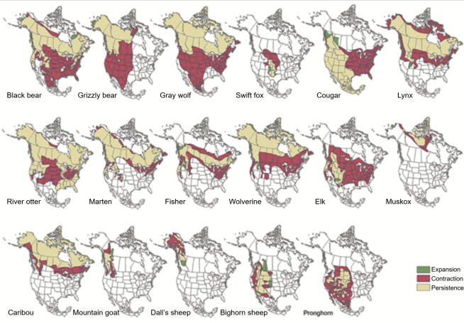
An important topic that will be analyzed is extirpation, otherwise known as local extinction. It is the concept of a species no longer appearing in a specific location, whether it died off or migrated elsewhere. For this study, a species will be considered locally extinct if it has not been observed in 2017. Inspiration to study this topic was from
Figure 1. which shows that numerous species’ populations are contracting in the state of Michigan. This figure was from 2004 which is why it was not used in forming any conclusions but it narrowed down what species to look at and to see if this trend continued.
As seen in the figure above, for the state of Michigan, the Gray wolf, Lynx, River Otter, Marten, Fisher, Wolverine, Elk, and Caribou had population contractions. There were no persistent or expanding populations in the state of Michigan which is worrisome.
2. Collected Data
The temperature data used in this research was sourced from the National Centers for Environmental Information (NCEI)
, a division of the National Oceanic and Atmospheric Administration (NOAA), specifically from the Muskegon County Airport's monthly temperature records. The dataset covers a substantial time frame, ranging from June 1896 to January 2025, allowing for a comprehensive analysis of long-term temperature trends in Muskegon County, Michigan. Temperature data for Stevens County, Minnesota; Spokane County, Washington; Nome Census Area County, Alaska; and Kennebec County, Maine were also observed to compare trends in other cold states. These counties were selected based on the amount of temperature data available for analysis. The start of the data range was from 1886 to 1906 with the end of this range being late 2024 to early 2025.
To make the data suitable for analysis, it was cleaned and converted from degrees Celsius to Fahrenheit. This conversion ensures consistency with other related temperature data and facilitates interpretation for a broader audience. In addition, any missing temperature data points were addressed by filling them using interpolation techniques. This imputation method ensures continuity in the dataset and reduces potential biases from missing data.
For the purpose of analyzing temperature patterns, the dataset was divided into five distinct time periods or ranges of years. This segmentation allows for a focused examination of temperature trends across different historical periods, providing insights into how temperature has changed over time and facilitating the detection of any emerging climate patterns. These temperature data will serve as the foundation for examining the potential correlation between temperature variations and changes in animal populations in cold states of the US.
The inputted data was a csv file that contained numerous variables related to the climate that were not used for this study and thus were removed. After getting rid of this information, converting the temperatures to Fahrenheit, and reformatting the data to be suitable for more types of chart, the output can be seen in
Table 1.
Table 1. Minimum Monthly Temperature in Degrees Fahrenheit In Muskegon County, Michigan. Minimum Monthly Temperature in Degrees Fahrenheit In Muskegon County, Michigan. Minimum Monthly Temperature in Degrees Fahrenheit In Muskegon County, Michigan.
Month | Jan | Feb | Mar | Apr | May | Jun | Jul | Aug | Sep | Oct | Nov | Dec |
1896 | | | | | | 44.96 | 50 | 42.08 | 30.92 | 24.98 | 12.92 | 10.04 |
1897 | -0.94 | 6.08 | -11.02 | 17.96 | 33.98 | 39.02 | 57.02 | 44.06 | 37.94 | 32 | 14 | 3.02 |
1898 | 10.04 | -4 | 6.08 | 17.96 | 35.96 | 42.98 | 48.02 | 51.08 | 37.94 | 30.92 | 5 | 5 |
1899 | -5.08 | -29.92 | 3.02 | 14 | 39.02 | 44.96 | 48.92 | 51.08 | 33.98 | 26.96 | 24.98 | 3.02 |
1900 | -0.94 | -0.94 | 3.92 | 24.98 | 32 | 42.08 | 50 | 57.02 | 37.04 | 32 | 15.98 | 5 |
1901 | -2.92 | -11.92 | 1.04 | 19.94 | 33.08 | 39.02 | 55.04 | 48.92 | 35.96 | 28.94 | 21.92 | -2.92 |
1902 | -2.02 | -11.02 | 8.06 | 19.04 | 32 | 42.98 | 46.94 | 46.04 | 39.92 | 30.92 | 24.98 | 8.96 |
… | … | … | … | … | … | … | … | … | … | … | … | … |
2020 | 15.26 | 9.14 | 16.16 | 24.26 | 23.18 | 42.08 | 55.04 | 48.92 | 37.04 | 29.12 | 24.26 | 16.16 |
2021 | 10.22 | -8.86 | 14.18 | 17.24 | 29.12 | 44.06 | 48.92 | 53.96 | 44.06 | 30.2 | 19.22 | 18.14 |
2022 | 2.12 | 3.2 | 14.18 | 25.16 | 37.94 | 44.06 | 53.06 | 51.98 | 39.02 | 31.1 | 22.1 | 7.16 |
2023 | 11.12 | 10.22 | 18.14 | 23.18 | 35.96 | 44.96 | 55.94 | 46.94 | 46.04 | 26.24 | 20.12 | 26.24 |
2024 | -0.76 | 15.26 | 18.14 | 32 | 41 | 42.08 | 46.04 | 50 | 42.08 | 29.12 | 25.16 | 12.2 |
2025 | 2.12 | | | | | | | | | | | |
As seen in the
Table 1 above, the monthly minimum temperature data in degrees Fahrenheit for 1896 to 2025 is kept in the cleaned data. Data between 1903 and 2019 were omitted from this figure for brevity.
Data related to observations of endangered species in Muskegon County, Michigan, was obtained from Michigan State University and sorted by observation date in ascending order
. This same process was done for Washington which had statewide data on the last observation dates for plants considered extirpated up to 1980
. For the other states, no publicly available data containing the last observation dates and locations for extirpated species could be found. Some states like Minnesota have this data only accessible to employees of their Department of Natural Resources to prevent poaching of these rare species
. Due to this, the state status of species was analyzed in these states for possibly extirpated and extirpated species.
To support conservation planning and biodiversity assessment efforts,
Table 2 presents a summary of rare, threatened, and special concern species observed in the county. It lists each species by its scientific and common name, followed by its conservation status at both the state (Michigan) and global levels. The table includes the State Status (e.g., Threatened (T), Special Concern (SC)), Global Rank and State Rank as defined by NatureServe's conservation status ranking system, indicating each species’ relative risk of extinction. Also provided are the number of known occurrences within the county and the year of the most recent recorded observation. This information offers insight into local biodiversity trends, highlights species that may require monitoring or protection, and illustrates the temporal range of documented sightings.
Table 2. Conservation Status and County Occurrence Records of Rare and State-Listed Plant and Animal Species (Last Observed 1898-2024). Conservation Status and County Occurrence Records of Rare and State-Listed Plant and Animal Species (Last Observed 1898-2024). Conservation Status and County Occurrence Records of Rare and State-Listed Plant and Animal Species (Last Observed 1898-2024).
Scientific Name | Common Name | State Status | Global Rank | State Rank | Occurrences in County | Last Observed in County |
|
Rorippa aquatica | Lake cress | SC | G4? | S2 | 1 | 1898 |
Lithospermum latifolium | Broad-leaved puccoon | SC | G4 | S2 | 1 | 1899 |
Triphora trianthophora | Nodding pogonia or three birds orchid | T | G4? | S1 | 1 | 1899 |
Euphorbia commutata | Tinted spurge | T | G5 | S1 | 1 | 1901 |
… | … | … | … | … | … | … |
Glyptemys insculpta | Wood turtle | T | G2G3 | S2 | 11 | 2024 |
Lithobates palustris | Pickerel frog | SC | G5 | S3S4 | 3 | 2024 |
Pantherophis spiloides | Gray rat snake | SC | G4G5 | S2S3 | 4 | 2024 |
Plebejus samuelis | Karner blue | T | G1G2 | S2 | 37 | 2024 |
Terrapene carolina carolina | Eastern box turtle | T | G5T5 | S2S3 | 26 | 2024 |
To effectively evaluate the conservation priority of species, it is critical to understand the global conservation status ranking system used by organizations such as NatureServe and the International Union for Conservation of Nature (IUCN). These Global Ranks (G-ranks) provide a standardized method for assessing a species’ risk of extinction across its entire range. Each rank, from G1 (Critically Imperiled) to G5 (Secure), is determined by multiple criteria, including the total number of known populations or occurrences, population trends, habitat condition, geographic range, and existing threats. The system enables researchers, conservationists, and policymakers to make informed decisions about resource allocation, recovery efforts, and biodiversity protection strategies. These ranks are especially important in regions undergoing rapid environmental change, where even minor shifts in habitat conditions can disproportionately affect vulnerable species.
Table 3 summarizes the definitions of global ranks used throughout this report to classify species based on their relative conservation concern.
Table 3. Global Conservation Status Ranks (G1-G5) and Their Definitions Based on Rarity and Extinction Risk. Global Conservation Status Ranks (G1-G5) and Their Definitions Based on Rarity and Extinction Risk. Global Conservation Status Ranks (G1-G5) and Their Definitions Based on Rarity and Extinction Risk.
| Global Rank |
G1 | Critically imperiled globally because of extreme rarity (5 or fewer occurrences range-wide or very few remaining individuals or acres) or because of some factor(s) making it especially vulnerable to extinction. |
G2 | Imperiled globally because of rarity (6 to 20 occurrences or few remaining individuals or acres) or because of some factor(s) making it very vulnerable to extinction throughout its range. |
G3 | Either very rare and local throughout its range or found locally (even abundantly at some of its locations) in a restricted range (e.g. a single western state, a physiographic region in the East) or because of other factor(s) making it vulnerable to extinction throughout its range; in terms of occurrences, in the range of 21 to 100. |
G4 | Apparently secure globally, though it may be quite rare in parts of its range, especially at the periphery. |
G5 | Demonstrably secure globally, though it may be quite rare in parts of its range, especially at the periphery. |
To complement global conservation assessments, state-level conservation status ranks—referred to as State Ranks (S-ranks)—are used to evaluate the rarity and threat levels of species within specific geographic boundaries. These ranks are essential for guiding local conservation efforts, land-use planning, and species management strategies. They consider factors such as the number of known occurrences within the state, population health, habitat condition, and specific threats that may not be reflected in global assessments. The ranks range from S1 (Critically Imperiled) to S4 (Apparently Secure) and help conservation agencies prioritize protection actions at the state or regional level.
Table 4 outlines the definitions and criteria used for each S-rank category.
Table 4. State Conservation Status Ranks (S1-S4) and Their Definitions Based on Local Rarity and Extirpation Risk. State Conservation Status Ranks (S1-S4) and Their Definitions Based on Local Rarity and Extirpation Risk. State Conservation Status Ranks (S1-S4) and Their Definitions Based on Local Rarity and Extirpation Risk.
| State Rank |
S1 | Critically imperiled in the state because of extreme rarity (5 or fewer occurrences or very few remaining individuals or acres) or because of some factor(s) making it especially vulnerable to extirpation in the state. |
S2 | Imperiled in state because of rarity (6 to 20 occurrences or few remaining individuals or acres) or because of some factor(s) making it very vulnerable to extirpation from the state. |
S3 | Rare or uncommon in state (on the order of 21 to 100 occurrences). |
S4 | Apparently secure in state, with many occurrences. |
3. Temperature Data Analysis For Michigan
The temperature distribution for each time period is depicted using radar charts, which represent the monthly temperature variations over a 12-month period. These charts visually illustrate the data as a temperature ring. The data presented in these graphs are based on the absolute minimum temperatures recorded each month. The term "absolute minimum" will be used when referring to the lowest of these minimum temperatures, while "temperature" will be used for brevity when referring to the minimum temperature itself. In the radar graph, the outer boundary of the ring corresponds to the maximum of the recorded minimum temperatures for each month, while the inner boundary represents the minimum of the recorded minimum temperatures.
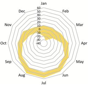
Figure 2. Radar Chart of the Minimum Temperatures in Degrees Fahrenheit from 1896 to 1920 for Muskegon County, Michigan. Radar Chart of the Minimum Temperatures in Degrees Fahrenheit from 1896 to 1920 for Muskegon County, Michigan.
Figure 2, covering the period from 1896 to 1920, illustrates significant fluctuations in minimum temperatures across the year. February recorded the lowest minimum temperatures, fluctuating between -30 and 10 degrees Fahrenheit. January followed closely, with temperatures ranging from -20 to 10 degrees Fahrenheit. The temperature distribution then began to increase, with March showing a range of -8 to 12 degrees, and December falling between -10 and 12 degrees.
In contrast, November had a wider range of 8 to 28 degrees, while April exhibited a broader variation between 12 and 30 degrees Fahrenheit. The months of October and May experienced more moderate temperatures, with ranges between 20 to 33 degrees Fahrenheit and 28 to 39 degrees Fahrenheit, respectively.
June marked a significant increase, with temperatures ranging from 40 to 51 degrees Fahrenheit, while September saw a range of 30 to 41 degrees. August, a warm month, exhibited temperatures from 40 to 58 degrees Fahrenheit, and July, the hottest month, recorded the highest variation, ranging from 43 to 58 degrees Fahrenheit.
These variations in temperature highlight the seasonal shifts and fluctuations, with the coldest temperatures occurring in winter and the warmest in summer, reflecting typical climate patterns.
Figure 3. Radar Chart of the Minimum Temperatures in Degrees Fahrenheit from 1921 to 1945 for Muskegon County, Michigan. Radar Chart of the Minimum Temperatures in Degrees Fahrenheit from 1921 to 1945 for Muskegon County, Michigan.
Figure 3 illustrates the variation in minimum temperatures for the period between 1921 and 1945. February emerged as the coldest month, with temperatures ranging from -14 to 10 degrees Fahrenheit. Following February, March recorded the next coldest temperatures, varying between -10 and 22 degrees Fahrenheit. January temperatures ranged from -4 to 15 degrees Fahrenheit, while December showed a similar range of -4 to 21 degrees Fahrenheit.
November's temperatures varied from 6 to 28 degrees, reflecting a relatively mild but still chilly range. April exhibited temperatures ranging from 10 to 30 degrees, while October saw temperatures from 23 to 38 degrees.
As the year progressed into the warmer months, May had a range of 28 to 43 degrees, and September ranged from 30 to 45 degrees. June temperatures varied from 35 to 48 degrees, signaling the beginning of the warmer season. Both August and July were the warmest months, with temperatures ranging from 40 to 55 degrees Fahrenheit.
These variations demonstrate the expected seasonal temperature shifts, with colder temperatures in the winter months and warmer temperatures during the summer months, with a slight overlap in the spring and fall.
Figure 4. Radar Chart of the Minimum Temperatures in Degrees Fahrenheit from 1946-1970 for Muskegon County, Michigan. Radar Chart of the Minimum Temperatures in Degrees Fahrenheit from 1946-1970 for Muskegon County, Michigan.
For the time period of 1946 to 1970 illustrated in
Figure 4, we can see that November was the coldest month with a range of -24 to 26 degrees Fahrenheit. January was the second coldest month with a range of -12 to 9 degrees with February being very similar with temperatures from -12 to 10 degrees. March ranged from -3 to 21 degrees followed by April which ranged from 17 to 28 degrees. May had temperatures from 22 to 40 degrees and September had temperatures ranging from 29 to 32 degrees. June had temperatures from 37 to 50 degrees and August had temperatures from 41 to 51 degrees. July was the hottest month with temperatures ranging from 42 to 53 degrees Fahrenheit.
Figure 5. Radar Chart of the Minimum Temperatures in Degrees Fahrenheit from 1971 to 2000 for Muskegon County, Michigan. Radar Chart of the Minimum Temperatures in Degrees Fahrenheit from 1971 to 2000 for Muskegon County, Michigan.
Data presented in
Figure 5 for the period of 1971 to 2000, the coldest month was February which had temperatures ranging from -20 to 19 degrees Fahrenheit. December was similar, ranging from -14 to 18 degrees while January ranged from -10 to 15 degrees. March ranged from -5 to 21 degrees and April ranged from 0 to 28 degrees. November had temperatures from 7 to 29 degrees and October ranged from 20 to 33 degrees. May had temperatures between 27 and 42 degrees while September ranged from 29 to 42 degrees. June ranged from 31 to 50 degrees while August had temperatures from 38 to 52 degrees. The hottest month was July which had temperatures from 41 to 52 degrees Fahrenheit.
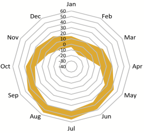
Figure 6. Radar Chart of the Minimum Temperatures in Degrees Fahrenheit from 2001 to 2025 for Muskegon County, Michigan. Radar Chart of the Minimum Temperatures in Degrees Fahrenheit from 2001 to 2025 for Muskegon County, Michigan.
Based on the temperatures recorded during the period of 2001 to 2025 illustrated in
Figure 6, the coldest month was January with temperatures between -11 and 18 degrees Fahrenheit. February was warmer than January with temperatures ranging from -8 to 15 degrees while December ranged from -5 to 18 degrees. March ranged from -5 to 20 degrees while November had temperatures between 14 and 19 degrees. April had temperatures from 16 to 32 degrees and May ranged from 25 to 41 degrees. October ranged from 27 to 35 degrees while September ranged from 34 to 50 degrees. June ranged from 36 to 50 degrees while July ranged from 40 to 59 degrees. The hottest month was August which ranged from 41 to 55 degrees Fahrenheit.
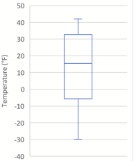
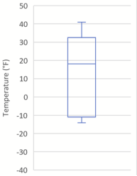
Figure 7. Box Plot of Minimum Temperatures in Degrees Fahrenheit from 1896 to 1920 for Muskegon County, Michigan. Box Plot of Minimum Temperatures in Degrees Fahrenheit from 1896 to 1920 for Muskegon County, Michigan.
Figure 7, summarizes the temperatures using Box Plot and this figure shows the absolute minimum temperature during the period of 1896 to 1920 was -30 degrees Fahrenheit while the highest temperature was 42 degrees. The median was 15 degrees and the lower and upper quartiles were -6 and 32 degrees respectively.
Figure 8. Box Plot of Minimum Temperatures in Degrees Fahrenheit from 1921 to 1945 for Muskegon County, Michigan. Box Plot of Minimum Temperatures in Degrees Fahrenheit from 1921 to 1945 for Muskegon County, Michigan.
The absolute minimum temperature during the period of 1921 to 1945 was -16 degrees Fahrenheit while the highest temperature was 40 degrees. The median was 15 degrees and the lower and upper quartiles were -5 and 32 degrees respectively as illustrated in
Figure 8.
Figure 9. Box Plot of Minimum Temperatures in Degrees Fahrenheit from 1946 to 1970 for Muskegon County, Michigan. Box Plot of Minimum Temperatures in Degrees Fahrenheit from 1946 to 1970 for Muskegon County, Michigan.
The Box Plot shown in
Figure 9 illustrated the absolute minimum temperature that was -14 degrees Fahrenheit during the period of 1946 to 1970 while the highest temperature was 41 degrees at the same period. The median was 19 degrees and the lower and upper quartiles were -11 and 32 degrees respectively.
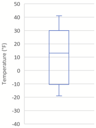
Figure 10. Box Plot of Minimum Temperatures in Degrees Fahrenheit from 1971 to 2000 for Muskegon County, Michigan. Box Plot of Minimum Temperatures in Degrees Fahrenheit from 1971 to 2000 for Muskegon County, Michigan.
During the period of 1971 to 2000, the absolute minimum temperature was -19 degrees Fahrenheit while the highest temperature was 41 degrees. The median was 12 degrees and the lower and upper quartiles were -10 and 30 degrees respectively as shown in the Box Plot presented in
Figure 10.
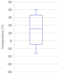
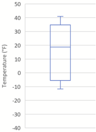
Figure 11. Box Plot of Minimum Temperatures in Degrees Fahrenheit from 2001 to 2025 for Muskegon County, Michigan. Box Plot of Minimum Temperatures in Degrees Fahrenheit from 2001 to 2025 for Muskegon County, Michigan.
Based on the recorded temperature illustrated in
Figure 11, the absolute minimum temperature during the period of 1971 to 2000 was -19 degrees Fahrenheit while the highest temperature was 41 degrees. The median was 19 degrees and the lower and upper quartiles were -5 and 35 degrees respectively.
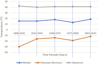
Figure 12. Minimum Temperatures in Degrees Fahrenheit Over Time for Muskegon County, Michigan. Minimum Temperatures in Degrees Fahrenheit Over Time for Muskegon County, Michigan.
The analysis compares absolute minimum, median, and maximum temperature values across five sequential 25-year intervals, spanning from 1896-1920 to 2001-2025 as shown in
Figure 12 and
Figure 13 The focus is to understand how temperature extremes and averages have changed over time, particularly in cold-adapted regions such as Michigan and other northern U.S. states.
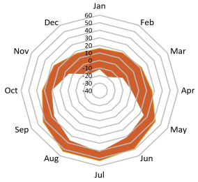
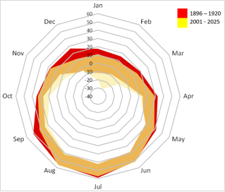
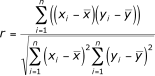
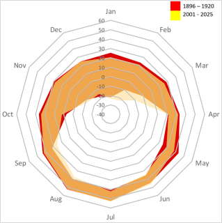
Figure 13. Radar Chart of 1896-1920 Temperatures on Top of 2001-2025 Temperatures in Degrees Fahrenheit for Muskegon County, Michigan. Radar Chart of 1896-1920 Temperatures on Top of 2001-2025 Temperatures in Degrees Fahrenheit for Muskegon County, Michigan.
A prominent finding is the significant increase in absolute minimum temperatures, which rose by approximately 18.2°F over the study period. This indicates that the coldest days of the year have become substantially milder over the past century. Such a shift is ecologically important because many species—especially those adapted to harsh winter conditions—depend on consistently cold temperatures for hibernation, breeding, or food availability. Warmer minimums may disrupt these life cycles and contribute to range shifts or population declines.
By contrast, median and maximum temperatures do not show a similarly strong or consistent trend. This suggests that while overall warming may be modest or variable during average or peak heat periods, the most profound and consistent change is occurring at the coldest extremes. These warming minimums could lead to decreased snowpack duration, altered frost timing, and increased winter precipitation as rain rather than snow—all of which have cascading ecological impacts.
This trend supports the argument that minimum temperature data should be included alongside average and maximum values when evaluating climate change impacts on ecosystems, especially in cold-weather regions.
In the
Figure 13, a comparison of
Figures 2 and 6 showing how the temperature shifted over 100 years where red represents the period of 2001-2025 light yellow represents the period of 1896-1920, and orange is the intersection of both these periods. The most noticeable change is February where the minimum temperature changes from -30 to -11 degrees Fahrenheit. Another noticeable trend can be seen in the fall where September’s absolute minimum temperature increased by about 5 degrees and October and November increased by around 8 degrees.
4. Animal Data Analysis for the State of Michigan
For the state of Michigan, no comprehensive dataset on animal populations could be found. This lack of data is due to surveying being a resource and time-intensive task, but Michigan State University provides a comprehensive list on endangered species and when they were last observed by county
.
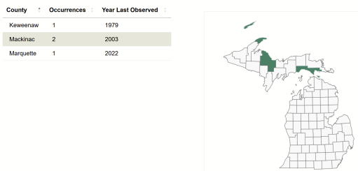
According to Michigan State University the last sighting of a Lynx in Michigan was in 2022 in Marquette County as shown in
Figure 14, followed by 2 occurrences in 2003 in Mackinac and 1 occurrence in Keweenaw County in 1979
.
As seen in the figure above, Lynx have only been observed in the Upper Peninsula, where only 1 occurrence was observed in 2022 in Marquette County. No new occurrences have been observed in Mackinac since 2003 and none in Keweenaw since 1979. This lack of new observations in Mackinac and Keweenaw Counties suggests that the Lynx populations died off or migrated elsewhere.
Another animal with a significant decline in population is the snowshoe hare
| [2] | Burt, D. M., G. J. Roloff, and D. R. Etter. 2016. “Climate Factors Related to Localized Changes in Snowshoe Hare (Lepus Americanus) Occupancy.” Canadian Journal of Zoology 95 (1): 15–22. https://doi.org/10.1139/cjz-2016-0180 |
[2]
. Surveys conducted by Michigan State University found with 95% accuracy “that hare populations experienced localized extinction on 52 sites (39%) statewide. In the northern Lower Peninsula, 36 of 74 sites (~49%) were unoccupied during 2013. Only 16 out of 60 (~27%) sites were unoccupied in the Upper Peninsula.” (Burt 2014).
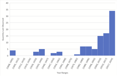
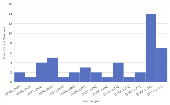
Figure 15. Dates of Muskegon County, Michigan Species Last Observed. Dates of Muskegon County, Michigan Species Last Observed.
Figure 15 shows the distribution of species last observed in Muskegon County, the county that the temperature data is from. Of the 105 species observed in Muskegon, 34 were last observed between 2017 and 2024. What's concerning is that 71 of these species have not been observed in the last 7 years, which is 67.6 percent of all species originally observed in Muskegon. The vast majority of these observations were between 1975 and 2017, which contains 52 observations, 72.2 percent of the observations before 2017, and 49.5 percent of the total observations (“Muskegon County Element Data.” 2024).
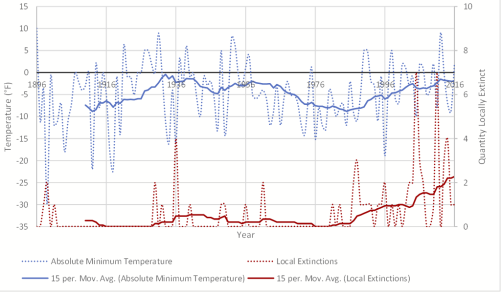
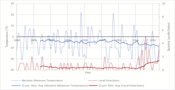
Figure 16. Minimum Temperatures vs. Local Extinctions for Muskegon County, Michigan.
The absolute minimum temperature and local extinctions over time are presented in
Figure 16. A simple moving average of 15 was used for the trendline of both datasets to smooth out the large amounts of fluctuations. What particularly stands out is the shape of both trendlines after 1976 where they both seem to increase at nearly identical linear rates. This strongly suggests that there is a correlation between absolute minimum temperature and local extinctions.
To get a mathematical relationship between the absolute minimum temperature and local extinctions in Muskegon County, Michigan, Pearson’s Correlation Coefficient Formula was used
Figure 17. This formula outputs a number between -1 and 1 where 1 means a perfect linear correlation, -1 means a perfect inverse linear relationship, and 0 means no relationship at all. The first correlation coefficient calculated was done on the original data which yielded a value of -0.11. This would mean there is an extremely weak negative correlation between temperature and local extinctions but this does not look like the case in
Figure 17 where there appears to be a fairly strong positive correlation.
Figure 17. Pearson’s Correlation Coefficient Formula. Pearson’s Correlation Coefficient Formula.
The reason this correlation is so low is due to large variation in both temperature and local extinctions which creates inconsistencies in point by point change. To address this issue, the data was smoothed with a simple moving average of 15 using the formula shown in
Figure 17. This same simple moving average was used to create the trendlines in
Figure 16 to make it easier to follow the trend in temperature and local extinctions.
This created a much more reasonable correlation of 0.40 which means that there is a relationship between temperature and local extinctions but it is not strong. For even further analysis, the correlation was calculated from 1976 to 2016 where
Figure 16 visually showed a strong correlation. This yielded a correlation coefficient of 0.92 which means that there is an extremely strong positive correlation between temperature and local extinctions.
5. Temperature Data Analysis for Alaska, Maine, Minnesota, and Washington
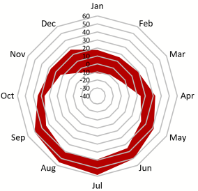
An expanded analysis of temperature trends across four additional U.S. states—Alaska, Maine, Minnesota, and Washington—selected for their ecological relevance and geographic diversity. These regions, like Michigan, harbor numerous cold-adapted species and have experienced varying degrees of climate change impacts. By examining long-term minimum monthly temperature records in these states, this analysis aims to contextualize Michigan’s trends within a broader national framework. This comparative approach helps identify whether similar warming patterns and potential risks to biodiversity are observable across other northern habitats.
As illustrated in
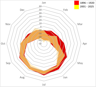
Figure 18, the notable changes in minimum temperature for the state of Alaska can be seen in January, February, March, April, August, and December. All but March increased in temperature by 5 to 10 degrees Fahrenheit while March decreased by 5 degrees. There are significant increases in minimum temperatures for February, April, May, and June, which increase by 19, 17, 6, and 7 degrees respectively.
Figure 18. Radar Chart of 1906-1920 Temperatures on Top of 2001-2025 Temperatures in Degrees Fahrenheit for Nome Census Area County, Alaska. Radar Chart of 1906-1920 Temperatures on Top of 2001-2025 Temperatures in Degrees Fahrenheit for Nome Census Area County, Alaska.
The radar chart presented in
Figure 19, the state of Maine has undergone tremendous changes in both minimum and maximum temperatures. The most notable change is the month of May where the minimum temperature increases by 45 degrees Fahrenheit. January, April, June, and July increase minimum temperatures by 20, 22, 35, and 27 degrees respectively. March, August, and November had an increase in minimum temperatures by 5 to 10 degrees Fahrenheit while September and October had no noticeable changes. February, October, November, and December all had warmed in maximum temperatures by approximately 20 degrees Fahrenheit.
Figure 19. Radar Chart of 1886-1920 Temperatures on Top of 2001-2025 Temperatures in Degrees Fahrenheit for Kennebec County, Maine. Radar Chart of 1886-1920 Temperatures on Top of 2001-2025 Temperatures in Degrees Fahrenheit for Kennebec County, Maine.
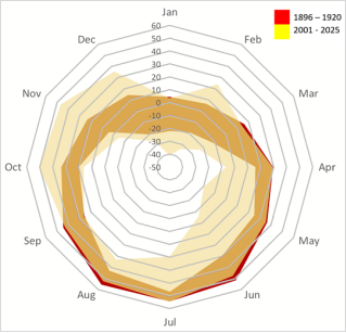
Figure 20. Radar Chart of 1886-1920 Temperatures on Top of 2001-2025 Temperatures in Degrees Fahrenheit for Stevens County, Minnesota. Radar Chart of 1886-1920 Temperatures on Top of 2001-2025 Temperatures in Degrees Fahrenheit for Stevens County, Minnesota.
Figure 20 shows that there is a noticeable increase in minimum temperatures for every month except April by about 5 degrees Fahrenheit on average with November having a significant increase by 15 degrees. December had a large increase in maximum temperatures by 15 degrees Fahrenheit. There were no other significant changes in maximum temperatures.
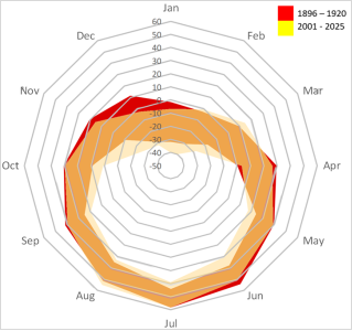
Figure 21. Radar Chart of 1889-1920 Temperatures on Top of 2001-2025 Temperatures in Degrees Fahrenheit for Spokane County, Washington. Radar Chart of 1889-1920 Temperatures on Top of 2001-2025 Temperatures in Degrees Fahrenheit for Spokane County, Washington.
As shown in the
Figure 21, February and March’s minimum temperatures both increased by around 10 degrees Fahrenheit. September’s minimum temperature increased by about 5 degrees Fahrenheit while May’s decreased by 5 degrees. January, February, March, and May all had an increase in maximum temperatures by 2 to 5 degrees Fahrenheit.
6. Organism Data Analysis for Alaska, Maine, Minnesota, and Washington
For the state of Washington, the date of extirpations for vascular plants was obtained from the Washington State Department of Natural Resources
. The State of Washington defined confident extirpation as being of species no longer being observed past 1980 which provided less data to compare with temperature overall.
In
Figure 22 the analysis results shows, 42%, or 21 of the 50 extirpations in the state of Washington occurred from 1967 to 1981, with no visible trend before 1967. This is a cause for concern as if that trend continues, there can be significant and further loss in biodiversity among plants.
Figure 22. Dates of Spokane County, Washington Vascular Plants Last Observed. Dates of Spokane County, Washington Vascular Plants Last Observed.
Figure 23. Minimum Temperatures vs. Local Extinctions in Washington. Minimum Temperatures vs. Local Extinctions in Washington.
While
Figure 23 shows absolute minimum temperatures decreased noticeably starting around 1956. Due to extirpation data for the state of Washington only containing species not observed past 1980, extirpations could not be compared with warming temperatures for the state of Washington.
Pearson’s correlation coefficient was calculated for the state of Washington with minimum temperatures and vascular plant extirpation to a result of -0.18923. Once again, this correlation is weak due to the large variations in both temperature and extirpation data. The calculation was redone with the simple moving averages for both variables for a correlation coefficient of -0.72431. This coefficient suggests that there is a strong negative correlation between minimum temperatures and vascular plant extirpations. This suggests that a decrease in temperature can cause harm to plant species. The state of Washington did not have overall major changes in temperatures, but in the last 25 years, February and March both significantly warmed by about 10 degrees Fahrenheit when compared to the earliest known data (See
Figure 21). If more extirpation data were available, comparisons could be done with a focus on these months' data to see how Washington’s plants correlate with warming temperatures.
The state of Washington has 6 animal species declared extirpated with 14 more considered possibly extirpated with the hope of rediscovery
. When compared to the state of Michigan, 21 local extinctions are relatively small versus the 71 in Michigan as shown in
Figure 15. Part of this discrepancy may be due to the far more lenient definition of local extinctions counting observations prior to 2017 versus 1980 for Washington. Another reason is likely due to the state of Washington having less variation in temperatures as shown in
Figure 21 when compared to Michigan
Figure 13.
Based on the Minnesota Star Tribune’s compilation of data from the Minnesota Department of Natural Resources, there have been 50 Plants and animals extirpated
. Minnesota had sizable increases in minimum temperatures for nearly every month when comparing the past 25 years to the earliest known temperature data shown in
Figure 20. This increase in temperatures and a large amount of extirpations supports the hypothesis.
According to the Maine Department of Agriculture, Conservation, and Forestry, there are 22 confirmed species of extirpated plants with 44 possibly extirpated plants
. Maine had the most significant changes in temperature with a 45-degree Fahrenheit increase in minimum temperature for the month of May shown in
Figure 19. Maine also defines species as extirpated if they have not been observed in the past 50 years but 66 extirpations are significant. This is 27% more than Washington which supports the hypothesis that increases in minimum temperatures harm animal populations.
The Alaska Department of Fish and Game (ADF&G) only mentions two species that have gone extinct, with both extinctions prior to 1906, the earliest temperature data analyzed in this study
. The ADF&G only lists 41 species that are federally endangered in the state of Alaska with only 11 of those species having critical habitats in Alaska
. This lack of extirpations and relatively low number of endangered species coincides with the low change in minimum temperatures seen in Alaska, supporting the hypothesis shown in
Figure 18.
7. Conclusion
For Muskegon County, Michigan, there is a significant increase in the minimum temperatures of 18.2 degrees Fahrenheit from the period of 1896 to 1920 to 2001 to 2025 as seen in
Figure 12. The most significant change was for the month of February which normally is the coldest month in Michigan. As time progressed, the absolute minimum temperature in February increased to the point of February having temperatures similar to January in the later periods, as seen in
Figures 2 and 6. There is also a significant increase in absolute minimum temperature for the fall with an average increase of 7 degrees Fahrenheit. For the state of Michigan, the increase in minimum temperatures supports the hypothesis that rising temperatures are a major cause of the decline of animal populations.
Furthermore, the increasing trend in local extinctions in the county of Muskegon is extremely worrying as seen in
Figure 7. Local extinctions seemed to accelerate at around 1976 at a similar time when temperatures seemed to start to rise significantly, with a total of 71 species becoming locally extinct. This trend correlates both visually, as seen in
Figure 16, and mathematically with temperature with a correlation of 0.92 past 1976 and an overall correlation of 0.4. This suggests that the increase in minimum temperatures is likely to have become a major cause of local extinctions around 1976, supporting the hypothesis of minimum temperature warming and organism population decline being correlated.
The other states analyzed on their own are not enough to form a conclusion due to the lack of data. When paired with the trends shown in Michigan, Alaska, Maine, and Minnesota support the hypotheses as the number of local extinctions looks to correlate with the changes in temperature. The state of Washington actually showed that temperature decreases caused extirpations in plants due to the observation cutoff being 1980 where there was a downward trend in temperature starting from 1965.
Another highlight of this research is the lack of overall plant and animal data available. States have different laws on data protection to prevent poaching, but data on endangered and extirpated species and when they were last observed is important information that should be publicly available. True population data for these species needs to be collected so trends can be analyzed and actions can be taken before the species goes locally extinct.
Based on the findings of this research, it is crucial that policies are put into place to slow down climate warming, and more effort is put into preserving these species. As biodiversity decreases due to extirpations, the whole ecosystem will suffer which can increase the spread of disease, cause food insecurity, as well as other economic damages.