Abstract
A tumor, otherwise called a neoplasm, are abnormal accumulations of tissues that can either be solid or filled with fluid. Lumps or growths known as tumors constitute clusters of abnormal cells, originating from any of the trillions of cells present throughout the body. The growth patterns and behaviors of tumors vary significantly, depending on whether their classification is cancerous (malignant), non-cancerous (benign) or precancerous. Medical imaging is a process that is widely used to produce images of the human body for both medical and research purposes. A significant focus in clinical research is the automated detection of tumors in the brain using Magnetic Resonance Imaging scans. Magnetic Resonance Imaging (MRI) is a sophisticated medical-imaging technology. It enables non-invasive visualization of the internal anatomy of the human body. Segmenting MRI images is vital for the detection of brain tumor. Complexities of tumor characteristics, such as shape and size, tumor-location, gray?level intensity, makes it challenging to classify segmented MRI scans into normal versus abnormal. Histogram Segmentation method, proposed in this study, is based on differentiating with order static filter. In post-processing, morphological techniques are practically employed to enhance the visibility of brain tumors. The K-Nearest Neighbors (KNN) classification method is then utilized to categorize tumor values into their respective categories, such as benign or malignant, based on the tumor's size. This approach helps patients and students to understand the tumor and helps physicians decide treatment based on the tumor’s size, shape, location and the type.
Keywords
Brain Tumors, MRI, Pre-processing, Order Static Filters, KNN Classification
1. Introduction
Tumors are a classic sign of inflammation and are either malignant (cancerous) or benign. The tissue-names where the tumors originate typically influence how they are named resulting dozens of names and types. These names sometimes also indicating their shape or growth characteristics. Each tumor is categorized by the names of the initially affected cells
.
Lumps or growths known as tumors constitute clusters of abnormal cells, originating from any of the trillions of cells present throughout the body. The growth patterns and behavior of tumors vary significantly, depending on whether they are classified as benign (non-cancerous), pre-cancerous, or malignant (cancerous)
.
Clinically, the broad classification of tumors falls under two types: primary and secondary. Tumors initially identified as primary remain localized to their area of origin and are sub-classified into benign and malignant types, while those that exhibit aggressiveness are referred to as secondary tumors.
Cancerous tumors
Cancer can originate in any area of the body, and when cancerous cells accumulate to form a lump or growth, it is termed a cancerous tumor. A tumor is considered cancerous if it:
1) invades nearby tissues
2) contains cells capable of detaching, traveling through the bloodstream or lymphatic system, and spreading to lymph nodes or distant parts of the body.
When cancer extends from its original location, named the primary tumor, to other regions of the body, it is said to be metastatic cancer. The newly formed tumors arising out of this spread are called metastases.
Tumors develop when dead cells accumulate and grow into a mass. While cancer cells grow in a similar fashion, they differ from the cells in benign tumors by their ability to invade surrounding tissues and disseminate throughout the body. Tumors represent a significant threat, as they can transform from normal cells into malignant growths, posing serious risks to human health. The deadlines of this tumors can be notified by the fact that converts to cancer stages and causes 10% of all the human deaths in 2016. Tumor mutation, the clinical term for which is malignancy, is a wide variety of disorders which involve unregulated cell growth. Uncontrolled division and growth of abnormal cells can lead to the formation of malignant tumors, which may invade surrounding tissues and potentially spread to other parts of the body via blood or the network of lymph vessels and nodes
. Not every tumor is cancerous; some are harmless. Benign tumors do not have uncontrolled growth, nor do they invade neighboring tissues, and remain localized.
Various techniques are employed to produce medical images for clinical studies, with MRI being the most commonly utilized. Compared to conventional imaging modalities such as X-rays and Computed Tomography (CT), which use high-energy ultraviolet (UV) radiation that can be harmful to the health of human beings, MRI scans rely on magnetic fields, which pose significantly fewer health risks. MRI images come in several modalities, in magnetic resonance imaging, different types of scans such as Sagittal, T1, T2, and FLAIR are used, each showing various aspects of the same organ. Research conducted by the American Brain Tumor Association
indicates that about 78,000 new cases are expected to be diagnosed, which includes 25,000 primary tumors and 53,000 non-malignant tumors.
2. Medical Background
Diagnosis and treatment largely depend on the tumor’s type and location. In some cases, benign tumors may require no intervention, while others may be surgically debulked (size reduction or completely removed. For malignant tumors, treatments often comprise of surgery, chemotherapy and radiation. Similarly other tumors include blastoma, desmoid tumor, ear tumor, epidermoid carcinoma, epithelial carcinoma, esophageal cancer, syringoma, fibroid, tumor marker etc.
. Not every tumor is cancerous; some are harmless. Benign tumors do not have uncontrolled growth, nor do they invade neighboring tissues, and remain localized. Tumor can be Benign (not cancerous) or malignant (cancerous). Cells within malignant tumors are abnormal and proliferate uncontrollably and chaotically. These cancerous cells have the ability to invade and damage tissues nearby, as well as spread to organs and body parts
.
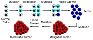
Figure 1. The development of a tumor encompasses multiple genetic mutations and the inactivation of tumor suppressor genes.
Figure 1 Cancer development requires numerous mutations to happen in a single- cell’s Deoxyribonucleic Acid (DNA). Initially, normal cells (light gray) in any of body’s organs may acquire mutations which enable mildly faster growth in them in comparison to surrounding cells. The mutated cells (light blue) are not yet considered tumor cells, as further mutations are required for the formation of cancer
. As these light blue mutated cells proliferate more rapidly, they create a 'larger' target for future mutations, increasing the likelihood of further genetic alterations on the path to cancer. Eventually, with the accumulation of sufficient mutations, the cells (dark blue) become a tumor, which remains non-malignant but will progress to malignancy if left untreated. The tumor cells continue to mutate, transforming into malignant cancer cells (red). These malignant cells form cancer in the original organ and will further accumulate mutations, eventually spreading (metastasizing) to other organs via the bloodstream.
3. Brain Tumor and Its Types
A brain tumor is among the most frequent and life-threatening diseases, with the potential to be fatal. Similar to other types of tumors, over 120 distinct types of brain tumors have been identified - some acute and others chronic. This study will focus on four specific types of brain tumors, as they are more severe and exhibit rapid growth
.
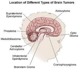
Figure 2. Location of various kinds of Brain tumors.
3.1. Glioblastoma (GBM)
These tumors develop in the brain's glial cells, thus classified as gliomas. One specific type is glioblastoma, also known as astrocytoma, which originates in the astrocytes.
3.2. Pinealomas
Pinealomas are considered primary tumors, with "pinealoma" being the term used for the most common type. The pineal gland's most frequently encountered tumors include germinomas, while other types consist of teratomas, pineocytomas, and pineoblastomas.
3.3. CNS Lymphoma
The form of tumor in the lymphatic tissues, which are been instrumental in the immune system of the body. Such type of cancer is identified as Central Nervous System (CNS) Central Nervous System Lymphoma (CNSL) or Primary Central Nervous System Lymphoma (PCNSL).
3.4. Metastatic
A metastatic brain tumor, also referred to as a secondary brain tumor, originates somewhere else in the body and subsequently spreads to the brain, leading to its development.
4. Magnetic Resonance Imaging (MRI)
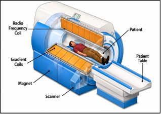
A magnetic resonance imaging (MRI) scanner uses great magnets to polarize and stimulate hydrogen nuclei (single proton) in human being tissues, which produces a signal that can be detected, and it is predetermined spatially
, ensuring in images of the body. Due to MRI technique, brain activity related to the blood can change due to the MRI techniques
Figure 3.
Figure 3. Magnetic resonance imaging (MRI), Scanner a narrow tube moves the patient through a tunnel.
Source: https://www.medicalequipment-msl.com/htm/medical-device-book/introduction-of-MRI.html
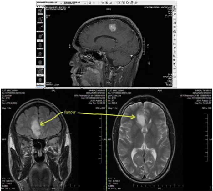
MRI can generate multiple planes or slices of the brain depending on the thickness and position of the head.
Figure 4 illustrates various slices and angles produced by different MRI modalities
. For diagnosing a specific type of brain tumor or disease, multiple modalities are used by physicians to thoroughly examine the nature of the condition.
| [6] | Seyed Matin Malakouti, Mohammad Bagher Menhaj, Amir Abolfazl Suratgar. “Machine learning and transfer learning techniques for accurate brain tumor classification” Distributed and Intelligent Optimization Research Laboratory, Department of Electrical Engineering, Amirkabir University of Technology, Tehran, Iran. Version of Record 10 August 2024. Clinical eHealth Volume 7, Pages 106-119, December 2024,
https://doi.org/10.1016/j.ceh.2024.08.001 |
| [7] | Oumaima Saidani, Nazik Alturki, Amal Alshardan, Turki Aljrees, Muhammad Umer, Sardar Waqar Khan, Shtwai Alsubai, Imran Ashraf, “Enhancing Prediction of Brain Tumor Classification Using Images and Numerical Data Features”, 13(15), 2544; DiagnosticsPublished: 31 July 2023
https://doi.org/10.3390/diagnostics13152544 |
[6, 7]
.
Figure 4. Brain MRI image and multiple modalities.
This research paper includes a review of the existing literature, followed by a detailed explanation of the methodology proposed for the study. The experimental results are then presented and discussed in depth. Finally, the paper concludes with a summary of the research findings.
5. Review of Literature
Angoth et al
introduced a wavelet-based fusion method for detecting brain tumors. In this approach, scans from diverse diagnostic techniques from CT and MRI, are processed using a median filter to enhance contrast and brightness. Following the filtering, the images undergo wavelet analysis and are subsequently fused by averaging the minimum or maximum of the wavelet coefficients. The proposed algorithm is benchmarked with other approaches to demonstrate its effectiveness.
Azhari et al
| [21] | E.-E. M. Azhari, M. M. M. Hatta, Z. Z. Htike, and S. L. Win, “Tumor detection in medical imaging: A survey,” International journal of Advanced Information Technology, vol. 4, Issue no. 1, p. 21, (2014). https://doi.org/10.5121/ijait.2014.4103 |
[21]
proposed a method for recognizing and detecting tumors in brain MRI images. To achieve higher-quality MRI images, a median filter is applied as a pre-processing step, followed by the canny edge detection method to smooth edges and identify their directions. The initial step involves using a histogram of clusters to construct the image and detect cancer. For system optimization, 50 scans were appropriated for training and 100 external neuroimaging tests were conducted, resulting in an 8% error rate for the proposed system.
Selva Kumar et al
| [22] | J. Selvakumar, A. Lakshmi, and T. Arivoli, “Brain tumor segmentation and its area calculation in brain images using k-mean clustering and fuzzy c-mean algorithm,” in Advances in Engineering, Science and Management (ICAESM), 2012 InternationalConferenceon., pp. 186–190. IEEE, 2012
https://ieeexplore.ieee.org/abstract/document/6215996 |
[22]
developed a methodology to segment brain tumors which leverages k-means and fuzzy C-means (FCM). To achieve more accurate results, salt-and-pepper noise is added to the median filter to suppress noise effectively. Characteristics are extracted using thresholding, and in the final step, an approximate reasoning method is employed to establish the shape and location of the tumor in MRI images. The method is evaluated against other segmentation algorithms and found to deliver higher accuracy in terms of segmentation.
Anam Mustaqeem et al
| [18] | Anam Mustaqeem, Ali Javed, Tehseen Fatima “An Efficient Brain Tumor Detection Algorithm Using Watershed & Thresholding Based Segmentation” I.J. Image, Graphics and Signal Processing, 10, pp -34-39. (2012)
https://www.researchgate.net/publication/266411344_ |
[18]
represented that Segmentation is main technique used. Out of different segmentation techniques, threshold segmentation, watershed segmentation and morphological operators used. The proposed segmentation method was experimented with MRI scanned images of human brains, thus locating a tumor in the images.
Fany Jesintha Darathi
| [32] | R.FanyJesintha Darathi, K.S.Archana, (2013) “Image Segmentation and Classification of MRI Brain Tumors Based on Cellular Automata and Neural Network” International Journal of Computational Engineering Research (ijceronline.com) Vol. 3 Issue. 3, march 2013, pp-323-327
https://www.ijceronline.com/papers/print-paper/3-3.pdf |
[32]
represented as out of different segmentation technique, seed based segmentation used and with this segmented image for detecting the tumor section and after that highlighting the region with help of level set method pre-processing.
Charutha S. et al
| [19] | Charutha S.M. J. Jayashree “An Efficient Brain Tumor Detection By Integrating Modified Texture Based Region Growing And Cellular Automata Edge Detection” IEEE, pp-1193-1199.“Radiopedia,”(2014)
https://ieeexplore.ieee.org/document/6993142 |
[19]
, presented an approach integrating edge detection using cellular automata combined with a modified texture-based region growing. Texture based region growing detected small sized tumor and cellular automata edge detection detected large sized tumor also modified in paper. Integration of these both techniques provides more efficient brain tumor detection.
Classification methodologies are employed to assign input data to separate categories, where validation are performed based on samples. KNN is extensively applied for categorizing tumors into relevant classes, e.g., tumor sub-structure, tumor, non-tumor, and malignant or benign
| [8] | MstSazia Tahosin, MdAlif Sheakh, RishalatunJannat Lima, Taminul Islam, Mahbuba Begum 3 “Optimizing brain tumor classification through feature selection and hyper parameter tuning in machine learning models” Informatics in Medicine Unlocked Volume43, 2023,
https://doi.org/10.1016/j.imu.2023.101414 |
| [9] | Aman Sharma “Brain Tumor Classification using Machine Learning and Deep Learning Algorithms: A Comparison: Classifying brain MRI images on the basis of location of tumor and comparing the various Machine Learning and Deep LEARNING models used to predict best performance.”, Pages 15 - 21 Published in IC3-2022: Proceedings of the 2022 Fourteenth International Conference on Contemporary Computing.
https://doi.org/10.1145/3549206.3549210 |
[8, 9]
.
The complexity of the structure of the brain makes segmenting a tumor a challenge. MRI scans are employed to thoroughly examine various parts of the body and are highly valuable for detecting early-stage brain abnormalities more effectively than other imaging techniques.
Brain tumor detection using MRI images has been extensively studied using both traditional image processing methods and advanced machine learning approaches
| [3] | Naeem, A., Senapati, B., & Zaidi, A. “Enhancing brain tumor detection from MRI-based images through deep transfer learning models”. 26 Nov, 2025,
https://doi.org/10.3390/ai6120305 |
| [5] | Fatma M. Refaat, M. M. Gouda and Mohamed Omar. “Detection and Classification of Brain Tumor Using Machine Learning Algorithms”. Biomedical & Pharmacology Journal, Vol. 15(4), p. 2381-2397. December 2022 https://biomedpharmajournal.org/vol15no4/detection-and-classification-of-brain-tumor-using-machine-learning-algorithms |
[3, 5]
. Recent developments in artificial intelligence, particularly deep learning, have significantly improved the accuracy of automated tumor detection systems.
6. Proposed Methodology
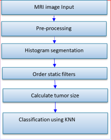
The methodology for developing a new technique focuses on the classifying and segmenting four basic tumor-types using multi-modal MRI images of the brain. This approach utilizes histogram differentiating for segmentation combined with unsupervised classification method such as KNN
. A rank filter is employed used in the post-processing phase, combined with morphological analysis to omit the skull and any extraneous particles from the segmented scans, facilitating easier calculations of the region of the tumor
| [18] | Anam Mustaqeem, Ali Javed, Tehseen Fatima “An Efficient Brain Tumor Detection Algorithm Using Watershed & Thresholding Based Segmentation” I.J. Image, Graphics and Signal Processing, 10, pp -34-39. (2012)
https://www.researchgate.net/publication/266411344_ |
[18]
. The size of the tumor will be determined over and done with matrix manipulation of the segmented image. Explains in the
Figure 5.
Figure 5. Flow of Algorithm for proposed method.
6.1. Sample Data Set
Table 1. Sample patient’s description.
Types of MRI Images | No of MRI Images | Patient Cases |
Glioblastoma | 25 | Male | 6 |
Female | 2 |
Pinealomas | 22 | Male | 3 |
Female | 2 |
CNS Lymphoma | 25 | Male | 2 |
Female | 4 |
Healthy | 25 | Male | 7 |
Female | 3 |
Metastases | 20 | Male | 4 |
Female | 1 |
The set of data employed, totaling 100 images, comprises of multiple modalities and variations of MRI images. These include both tumor-affected and image scans. Detailed information about the dataset is given in
Table 1. The dataset was compiled from online radiological sources, such as Radiopaedia
| [25] | Johnson DR, Guerin JB, Giannini C, Morris JM, Eckel LJ, Kaufmann TJ “2016 updates to the WHO brain tumor classification system: what the radiologist needs to know. Radio-graphics” 37: 2164–2180. (2017)
https://doi.org/10.1148/rg.2017170037 |
[25]
, and verified by a neurosurgeon to ensure its authenticity. The below
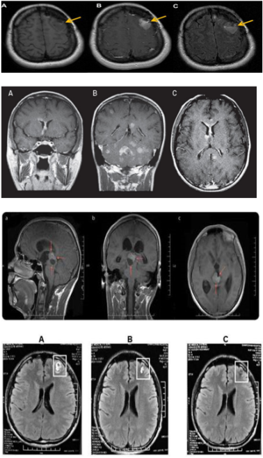
Figure 6 illustrates samples of our dataset for the specified tumor types.
Figure 6. Sample of MRI modalities and tumor types used in our dataset.
In
Figure 6(a), explains about male patient case whose age is above 65 years with the most prospective low-grade glioma or Glioblastoma (GBM) with major mass effect.
Figure 6(b), shows the presence of Primary CNS lymphoma coronal T1 post-contrast (A and B) and axial T1 Post-contrast (C) showing multiple and deep, cortical, and subcortical lesions that reach the genu of the corpus callosum. The second image (B) shows contrast enhancing nodules in the cerebellar parenchyma and leptomeningeal enhancement. There is also sub ependymal spread. The central nervous system involvement was secondary to no Hodgkin lymphoma of b-cell phenotype
| [32] | R.FanyJesintha Darathi, K.S.Archana, (2013) “Image Segmentation and Classification of MRI Brain Tumors Based on Cellular Automata and Neural Network” International Journal of Computational Engineering Research (ijceronline.com) Vol. 3 Issue. 3, march 2013, pp-323-327
https://www.ijceronline.com/papers/print-paper/3-3.pdf |
[32]
.
In
Figure 6(c), illustrations the MRI images of Pinealomas tumor which relates to women patient of Middle age with a unadorned headache. Pinealomas. The solid component only minimally enhances with a focal region demonstrating more prominent ring enhancement.
6.2. Pre-processing
Pre-processing steps adapt the image to meet the requirements for the subsequent analysis. This phase involves objects and noise filtering, in-image edge-sharpening, conversion of Red, Green, and Blue (RGB) images to grayscale, and reshaping of the images. Even though current MRI systems are technologically advanced to negate noise, it can still however occur due to thermal effect. Numerous filters exist for removal of noise such as order static filter. This study aims at detection and segmentation of tumors. A full-fledged system, however, requires noise-filtering. Generally Median filter is used to remove noise. The detected edges are added to the original image to enhance it edges. This makes tumor detection and segmentation easy
.
6.3. Histogram Based Segmentation
Segmentation of tumor region using semi-automated methods achieves acceptable outcomes over manual segmentation
| [7] | Oumaima Saidani, Nazik Alturki, Amal Alshardan, Turki Aljrees, Muhammad Umer, Sardar Waqar Khan, Shtwai Alsubai, Imran Ashraf, “Enhancing Prediction of Brain Tumor Classification Using Images and Numerical Data Features”, 13(15), 2544; DiagnosticsPublished: 31 July 2023
https://doi.org/10.3390/diagnostics13152544 |
[7]
. Semi-automated approaches may be broken down into three forms: initialization, evaluation, and feedback response.
Histogram-based segmenting relies on analyzing the image's histogram, so it's essential to prepare both the histogram and pertaining image beforehand. This approach uses the histogram to determine gray levels for grouping pixels into distinct regions. The two primary components in a basic image: the object and the background. The latter usually occupies the majority of the image and consists of a single gray level. The histogram is created by dividing the data range into equally sized bins or sections, denoted as classes. Then, for each bin, the count of data points contained within that range is counted. When constructing image histograms, the values corresponding to each pixel are charted along the horizontal axis
| [22] | J. Selvakumar, A. Lakshmi, and T. Arivoli, “Brain tumor segmentation and its area calculation in brain images using k-mean clustering and fuzzy c-mean algorithm,” in Advances in Engineering, Science and Management (ICAESM), 2012 InternationalConferenceon., pp. 186–190. IEEE, 2012
https://ieeexplore.ieee.org/abstract/document/6215996 |
[22]
.
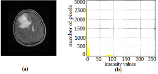
Initially, we generate a histogram relating to the original grayscale MRI scan.
Figure 7 illustrates the histogram corresponding to the original grayscale image.
Figure 7. a) The original grayscale image, b) histogram of the original grayscale image.
Once the generating of the grayscale-image’s histogram is done, the total column-count in the image is calculated to separate the left and right sections for histogram-based segmentation (HS). Computation of Separate histograms for the left and right sides is done to identify differences between the two. The steps involved in the histogram segmentation are as follows.
6.4. Histogram Based Segmentation Basic Steps
1) Find matrix M in gray scale image
2) Dive the matrix M by 2, m/2 for finding
3) left side of the image “LH” ❖ Right side of the image “RH”
4) Subtract LH and RH to find the difference of histogram “HS”
5) Apply Threshold T on HS to get the final difference image I.
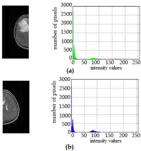
Figure 8(a) displays the left side of the initial grayscale scan alongside its corresponding histogram, which illustrates the grayscale pixel levels and the number of pixels at each level. Similarly,
Figure 8(b) shows the right side of the initial grayscale image with its respective histogram, presenting the grayscale pixel levels and pixel counts
| [10] | Sadia Maduri Rasa, Md. Manowarul Islam md, Md. Alamin Talukder, Md. Ashraf Uddin, Majdi Khalid, Mohsin Kazi, and Md. Zobayer Kazi.”Brain tumor classification using fine-tuned transfer learning models on magnetic resonance imaging (MRI) images”. Published online October 7, 2024,
https://doi.org/10.1177/20552076241286140 |
[10]
.
Figure 8. (a) The resulting histogram along with the left side of the initial grayscale image (b) The output histogram along with the right side of the initial grayscale image.
After the LH and RH of the original grayscale image, together with their corresponding histograms, are calculated from the initial MRI of the brain, the differences between LH and RH histograms, is then calculated.
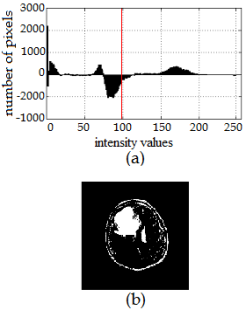
Computing the differences between the histograms outputs a segmented image that highlights the tumor-affected area within the MRI. The output image generated by histogram differentiating is shown in
Figure 9. In
Figure 9(a), the histogram represents the variances between the two histograms computed earlier, while
Figure 9(b) displays the segmented image, with tumor-affected area appearing as the foreground.
Figure 9. Presents the outcomes of histogram differentiating: (a) represents the resulting histogram obtained by subtraction of the two histograms, and (b) displays the image produced once the thresholding is applied to the generated image arising out of histogram differentiating.
6.5. Post-Processing Phase
In the post-processing phase, two techniques are combined—3-D order statistic filtering and morphological operations—to amplify the fidelity of the tumor-detection image. The 3-D order statistic filter is applied to assist the morphological operations by reducing the size of the structural element used for erosion and dilation
.
a) Order statistic filter
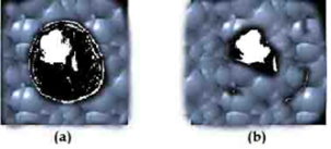
Figure 10 clearly demonstrates that extra boundaries can distort the shape and size of the detected tumor in the image obtained from histogram differentiating. To eliminate these unwanted boundaries, an Order Statistic Filter (OSF) is applied. OSF is an order-based filter that estimates different statistical measures, such as the minimum (first order) or maximum (largest order). Given a set of observations X1, X2, X3…………..X
N for a random variable X
. This process generates sorted values. This outputs Y(i) that satisfy X(1), X(2), X(3),…..X(N), where X represents the N observations processed by the OSF, thus, serving as an estimator for these sorted observations.
F(X1, X2, X3…...XN).
OSF filtration performs exceptionally well when added white noise or impulsive noise is present, given that the designing of the filter is appropriate. One of its key properties is the capability to preserve edges while maintaining simplicity in computations
, thus allowing faster computations when the algorithm is effectively structured. Following the application of the order statistic filter, the shape and size of the tumor become more distinct. The results of this filtering process are shown in
Figure 10, where the boundaries are removed without significantly altering the size and shape of the tumor, up to a certain extent
.
Figure 10. Illustrates the final output produced by the order-statistic filter.
(a) Displays the image obtained from histogram differentiating
(b) Shows the output image post OSF filtration
b) Dilation and erosion operation
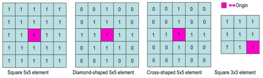
While applying OSF yields significant results, some residual noise may still impact the precision of tumor size calculations. To achieve exact delineation of the tumor for size measurement, morphological operations are employed to eliminate these minor noise artifacts and particles. OSF combined with morphology produces enhanced results. The structural elements designed for performing dilation and erosion operations are 5×5 for dilation and 3×3 for erosion.
Figure 11 illustrates the size and construction of the structural elements developed for this purpose, both of which deliver the desired results.
Figure 11. displays the two structuring elements (SE) employed during the dilation and erosion processes. Part (a) 5x5 diamond-shaped SE (b) 5×5 diamond-shaped SE (c) Cross-Shaped 5X5 Element.
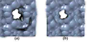
In
Figure 12, the tumor becomes more pronounced following the application of morphological erosion and dilation based on the designed structural elements. This enhancement facilitates the accurate calculation of tumor size and aids in classifying the tumor according to its dimensions.
Figure 12. Illustrates the final output image produced by morphology.
(a) The resultant of OSF in
Figure 7(b)(b) The final image output post morphology
7. Classification Using KNN
K-Nearest Neighbor (KNN) is a non-parametric algorithm, making it highly applicable to real-world problems for classification and regression tasks. It works by storing all instances and classifying new instances based on a similarity function, such as distance metrics like Euclidean distance, to find the nearest neighbors. KNN is a statistically-driven method applied for recognizing patterns and case classification
.
When it comes to continuous values, KNN applies various k values to measure and calculate the distance between two classes, typically using Euclidean distance for kk values in the range of 1 to 5. In this research, KNN classification is employed to categorize tumors into either malignant or benign. The classification utilizes tumor size values obtained from segmented images that highlight the tumor tissues
, with measurements representing different tumor sizes in square millimeters (mm
2). The said values are obtained for the entire image-dataset and further used for KNN classification.
For classifying the two categories, we use datasets labeled as 'a' and 'b,' representing the different classes (a1, b1),………………………., (an, bn).
a€RD, 'a' represents the values of the classes—tumor and non-tumor—plotted along the x-axis in a D-dimensional plane.
b € {0,1}, 'b' represents a finite set of classes used for classification, where the values are assigned to either the tumor or non-tumor category. When introducing a new value, 'z,' it serves as a label for a class determined by the k-nearest values, classifying the value into the appropriate category. If the majority of the labels closest to the k-nearest point 'z' belong to one class, the classification will result in that class being assigned as the resultant
| [4] | Musthafa, N., et al. “Advancing brain tumor analysis: Current Trends, Key Challenges and Perspectives in Deep Learning-Based Brain MRI Tumor Diagnosis”. 22 April 2025
https://doi.org/10.3390/eng6050082 |
[4]
.
In Region Growing (RG) approaches, image pixels form disjoint areas are analyzed through neighboring pixels, which are merged with homogeneousness characteristics based on pre-defined similitude criteria.
8. Results and Discussion
Following segmentation, the size of the tumor is calculated, and the tumor-percent within the MRI scan is determined. As per the 2007 World Health Organization (WHO) report
, tumor- classification ranges from grade 1 to grade 4, based on characteristics such as aggressiveness, intensity and size. Tumor-size is a key feature for categorizing tumors, aiding in the identification of the appropriate grade.
In this study, the tumor’s size and location is assessed using matrix manipulation (MM). The MM technique calculates the pixel-count of the foreground (tumor) and the background (non-tumor), providing an accurate measure of the tumor’s extent and magnitude.
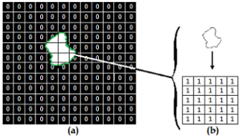
To determine both the pixel-count of both the background and foreground, the Total Number of Pixels (TNP) is estimated first to the final the segmented image from the given matrix. After obtaining the TNP using matrix manipulation (MM), we then calculate the Number of Foreground Pixels (NFP). In the matrix representation, foreground pixels are denoted by '1,' while background pixels are indicated by '0'.
Figure 13. Illustrates the segmented-image matrix, (a) represents a complete image-matrix of TNP, (b) represents the tumor / segmented area with its desire matrix for the calculation of NFP for the size of the tumor.
The Number of Foreground Pixels (NFP) represents the tumor pixels important for determining the tumor size. As illustrated in
Figure 13, the matrix of the segmented image illustrates the values of pixels of both foreground (tumor) and background
, using which are calculation of the size of the tumor is done. Once the TNP and NFP are computed from the image matrix, the tumor size is computed in two ways: as a percentage and in square millimeters (mm
2).
To estimate the tumor size as a percentage, the NFP is divided by the TNP, and the result is multiplied by 100, resulting in percentage size.
Mode 1: calculate the dimension of the tumor in percentages
IF
TNP = 8000 pixels
AND
NFP = 1200 pixels
THEN
Tumor size = NFP / TNP * 100
Tumor size = 1200/ 8000 *100
In the segmented MRI scan of the brain, the tumor appears to be 15% in size.
In method two of tumor size calculation, after determining the tumor’s size as a percentage, the same parameters obtained through Matrix Manipulation (MM) are utilized to compute the tumor size in square millimeters (mm2).
The steps to estimate the size of the tumor in square millimeters (mm2) in method two are detailed here. The first step is to take the square root of the NFP. Then, multiply the resulting value by the area represented by a single pixel, resulting in 0.264 mm2 (one pixel = 0.264 mm2). This calculation converts the size of the tumor from pixel units into a measurement in mm2, providing a more accurate representation of the tumor's actual size in the MRI image.
Mode 2: Tumor size in mm2
1 pixel = 0.264 mm2
Tumor size = | (√NFP)| * 0.264 mm2
IF
NFP = 1200
THEN
Tumor size = = | (√1200)| * 0.264 mm2
Tumor’s size is 9.15 mm
2 in the segmented brain MRI image. After determining the size of the tumor in square millimeters (mm
2) from the foreground-pixel computation, the values of the calculated size are employed for classification into two categories: benign and malignant. This classification process employs the K-Nearest Neighbor s (KNN) algorithm
| [31] | Park CR, Kim K, Lee Y “Development of a bias field-based uniformity correction in magnetic resonance imaging with various standard pulse sequences”. Optik 178: 161–166 population-and patient-specific feature sets. Computer Med Image Graph 37: 512–521(2019).
https://doi.org/10.1016/j.ijleo.2018.09.156 |
[31]
.
To classify the MRI images as either tumor-affected or healthy, size values for both classifications are computed. KNN uses the Euclidean Distance metric, and multiple k-values (ranging between 1 and 5) are considered to assess the algorithm's effectiveness in categorizing the MRI images accurately
| [34] | Shubhangi Solanki, Uday Pratap Singh, Siddharth Singh Chouhan, and Sanjeev Jain (2017) “Brain Tumor Detection and Classification using Intelligence Techniques: An Overview” IEEE(2017),
https://doi.org/10.1109/ACCESS.2023.3242666 |
[34]
.
To calculate the percentage of accuracy for the several k variations using the K-Nearest Neighbors (KNN) algorithm, the False Classification Rate (FCR) and True Classification Rate (TCR) are determined based on the dataset values.
Calculating FCR and TCR requires using the Total Number of False Classified Values (TNFCV) and Total Number of True Classified Values (TNTCV) out of the Total Number of Values (TNV) used for KNN for classification.
To calculate TCR:
TCR = (TNTCV /TNV) *100(1)
FCR = (TNFCV/TNV) *100(2)
To calculate FCR:
Table 2 presents the outcomes of KNN classification for varying k values. The dataset includes 50 patient cases, totaling 100 MRI images, comprising four tumor types and healthy samples. Classification outcomes may differ based on the dataset's characteristics and size, with kk values between 1 and 5 used for testing.
Table 2 shows that each k value results in a different classification rate. When k=1k=1, the True Classification Rate (TCR) is 95%, while for k=5k=5, the TCR increases to 99%. The results indicate that choosing a kk value greater than 5 might make possible biased outcomes for the given dataset. Testing suggests that the most suitable kk value lies between 1 and 5 for optimal performance.
Table 2 presents the overall True-Classification-Rate (TCR) and False-Classification-Rate (FCR) for the proposed dataset, based on k values between 1 and 5.
Table 2. Detail Description of TCR and FCR Based on K Values from 1 To 5.
k | 1 | 2 | 3 | 4 | 5 |
TCR | 95% | 96% | 97% | 98% | 99% |
FCR | 5% | 4% | 3% | 2% | 1% |
9. Conclusion
Tumors located in the brain refer to an abnormal mass within the brain, which can be classified as malignant or benign. The characteristics of these tumors, located in the brain, differ based on their location and size within the brain. Image processing is critical to the successful diagnosis and treatment of brain tumors, leveraging the advantages of the imaging technology of the MRI. This research has presented an approach to segment and classify four widely prevailing brain tumors. The dataset utilized in this study comprises of 100 MRI images, under the expertise of a neurosurgeon. To differentiate tumor pixels from surrounding brain tissue, a histogram-based segmentation approach was employed. Following this segmentation, the morphological operations and the order statistic filter were applied the technique like post-processing to improvises the results for segmentation results. After successfully differentiating the tumor region using histogram segmentation with MRI images, calculation of the tumor size is done. This is done through matrix manipulation in two distinct modes: percentage and mm2. The computed mm2 values are then used in the KNN classification to categorize tumors as malignant or benign. This classification approach relies on Euclidean distance and evaluates different variations of k values for testing and algorithm assessment. The average True Classification Rate (TCR) is 97%, while the average False Classification Rate (FCR) is 3% across the different k values.
10. Future Work
Future research can further enhance the proposed system in several ways. First, utilizing larger and more diverse medical datasets can improve the model’s ability to generalize across different cases. Additionally, integrating explainable techniques will help in visualizing tumor regions in MRI images, making the system more transparent and trustworthy for medical professionals. The development of real-time clinical decision support systems can also make this approach more practical for hospital use. Furthermore, extending the system to include tumor segmentation along with classification will provide more detailed diagnostic insights. Overall, future work will focus on improving model accuracy, reliability, and applicability in real-world medical settings.
Despite these advancements, several challenges remain, including dataset imbalance, model interpret ability, and generalization across different clinical datasets. Therefore, further research is required to develop more robust and reliable brain tumor detection systems using artificial intelligence techniques.
Abbreviations
MRI | Magnetic Resonance Imaging |
KNN | K-Nearest Neighbors |
CT | Computer Tomography |
UV | Ultra Violet |
DNA | Deoxyribonucleic Acid |
GBM | Glioblastoma |
CNS | Central Nervous System |
CNSL | Cashew Nut Shell Liquid |
PCNSL | Primary Central Nervous System Lymphoma |
FCM | Fuzzy C-Means |
RGB | Red, Green, Blue |
HS | Histogram Based Segmentation |
OSF | Order Statistic Filter |
SE | Structuring Elements |
RG | Region Growing |
WHO | World Health Organization |
MM | Matrix Manipulation |
TNP | Total Number of Pixels |
NFP | Number of Foreground |
FCR | False Classification Rate |
TCR | True Classification Rate |
TNFCV | Total Number of False Classified Values |
TNV | Total Number of Values |
Author Contributions
Pulipati Jyotsna: Conceptualization, Formal Analysis, Funding Acquisition, Methodology, Validation, Writing – original draft
Swathi Pothala: Conceptualization, Funding Acquisition, Methodology, Resources, Writing – original draft
Desineni Sudhakar: Formal Analysis, Funding Acquisition, Supervision, Validation
Kumba Vijaya Lakshmi: Data Curation, Funding Acquisition, Investigation, Methodology
Conflicts of Interest
The authors declare no conflicts of interest.
References
| [1] |
Wong, Y., et al. “Brain tumor classification using MRI images and deep learning techniques”.PLoSONE., Published: May 9, 2025,
https://doi.org/10.1371/journal.pone.0322624
|
| [2] |
Bouhafra, S., & El Bahi, H. “Deep learning approaches for brain tumor detection and classification using MRI images: A systematic review”.Sep30, 2024
https://doi.org/10.1007/s10278-024-01283-8
|
| [3] |
Naeem, A., Senapati, B., & Zaidi, A. “Enhancing brain tumor detection from MRI-based images through deep transfer learning models”. 26 Nov, 2025,
https://doi.org/10.3390/ai6120305
|
| [4] |
Musthafa, N., et al. “Advancing brain tumor analysis: Current Trends, Key Challenges and Perspectives in Deep Learning-Based Brain MRI Tumor Diagnosis”. 22 April 2025
https://doi.org/10.3390/eng6050082
|
| [5] |
Fatma M. Refaat, M. M. Gouda and Mohamed Omar. “Detection and Classification of Brain Tumor Using Machine Learning Algorithms”. Biomedical & Pharmacology Journal, Vol. 15(4), p. 2381-2397. December 2022
https://biomedpharmajournal.org/vol15no4/detection-and-classification-of-brain-tumor-using-machine-learning-algorithms
|
| [6] |
Seyed Matin Malakouti, Mohammad Bagher Menhaj, Amir Abolfazl Suratgar. “Machine learning and transfer learning techniques for accurate brain tumor classification” Distributed and Intelligent Optimization Research Laboratory, Department of Electrical Engineering, Amirkabir University of Technology, Tehran, Iran. Version of Record 10 August 2024. Clinical eHealth Volume 7, Pages 106-119, December 2024,
https://doi.org/10.1016/j.ceh.2024.08.001
|
| [7] |
Oumaima Saidani, Nazik Alturki, Amal Alshardan, Turki Aljrees, Muhammad Umer, Sardar Waqar Khan, Shtwai Alsubai, Imran Ashraf, “Enhancing Prediction of Brain Tumor Classification Using Images and Numerical Data Features”, 13(15), 2544; DiagnosticsPublished: 31 July 2023
https://doi.org/10.3390/diagnostics13152544
|
| [8] |
MstSazia Tahosin, MdAlif Sheakh, RishalatunJannat Lima, Taminul Islam, Mahbuba Begum 3 “Optimizing brain tumor classification through feature selection and hyper parameter tuning in machine learning models” Informatics in Medicine Unlocked Volume43, 2023,
https://doi.org/10.1016/j.imu.2023.101414
|
| [9] |
Aman Sharma “Brain Tumor Classification using Machine Learning and Deep Learning Algorithms: A Comparison: Classifying brain MRI images on the basis of location of tumor and comparing the various Machine Learning and Deep LEARNING models used to predict best performance.”, Pages 15 - 21 Published in IC3-2022: Proceedings of the 2022 Fourteenth International Conference on Contemporary Computing.
https://doi.org/10.1145/3549206.3549210
|
| [10] |
Sadia Maduri Rasa, Md. Manowarul Islam md, Md. Alamin Talukder, Md. Ashraf Uddin, Majdi Khalid, Mohsin Kazi, and Md. Zobayer Kazi.”Brain tumor classification using fine-tuned transfer learning models on magnetic resonance imaging (MRI) images”. Published online October 7, 2024,
https://doi.org/10.1177/20552076241286140
|
| [11] |
American brain tumor association,
http://www.abta.org/
|
| [12] |
Ali AH, Al-hadi SA, Naeemah MR, Mazher AN “Classification of brain lesion using K-nearest neighbor technique and texture analysis”. J Phys Conf Ser: 01 2018.
https://iopscience.iop.org/article/10.1088/1742-6596/1178/1/012018
|
| [13] |
American brain tumor association (glioblastoma), accessed: 2017-09-21 (2017)
http://www.abta.org/secure/glioblastoma-brochure.pdf
|
| [14] |
American brain tumor association (lymphoma), (2017), accessed: 2017-09-21.
http://www.abta.org/brain-tumor-information/types-of-tumors/
|
| [15] |
American brain tumor association (metastatic), (2017), accessed: 2017-09-21.
http://www.abta.org/secure/metastatic-brain-tumor.pdf
|
| [16] |
Amin J, Sharif M, Raza M, Saba T, Anjum MA “Brain tumor detection using statistical and machine learning method”. Comput Methods Progr Biomed 177: 69–79(2019)
https://www.sciencedirect.com/science/article/pii/S0169260718313786
|
| [17] |
Amin J, Sharif M, Yasmin M, Fernandes SL “A distinctive approach in brain tumor detection and classification using MRI”. Pattern Recogn Lett 139: 118–127(2020).
https://www.sciencedirect.com/science/article/pii/S016786551730404X
|
| [18] |
Anam Mustaqeem, Ali Javed, Tehseen Fatima “An Efficient Brain Tumor Detection Algorithm Using Watershed & Thresholding Based Segmentation” I.J. Image, Graphics and Signal Processing, 10, pp -34-39. (2012)
https://www.researchgate.net/publication/266411344_
|
| [19] |
Charutha S.M. J. Jayashree “An Efficient Brain Tumor Detection By Integrating Modified Texture Based Region Growing And Cellular Automata Edge Detection” IEEE, pp-1193-1199.“Radiopedia,”(2014)
https://ieeexplore.ieee.org/document/6993142
|
| [20] |
Despotovi ́c I, Goossens B, Philips W “MRI segmentation of the human brain: challenges, methods, and applications. Comput Math Methods” Med 2015: 1–23. (2015)
https://onlinelibrary.wiley.com/doi/full/10.1155/2015/450341
|
| [21] |
E.-E. M. Azhari, M. M. M. Hatta, Z. Z. Htike, and S. L. Win, “Tumor detection in medical imaging: A survey,” International journal of Advanced Information Technology, vol. 4, Issue no. 1, p. 21, (2014).
https://doi.org/10.5121/ijait.2014.4103
|
| [22] |
J. Selvakumar, A. Lakshmi, and T. Arivoli, “Brain tumor segmentation and its area calculation in brain images using k-mean clustering and fuzzy c-mean algorithm,” in Advances in Engineering, Science and Management (ICAESM), 2012 InternationalConferenceon., pp. 186–190. IEEE, 2012
https://ieeexplore.ieee.org/abstract/document/6215996
|
| [23] |
Javaria Amin; Muhammad Sharif; Anandakumar Haldorai; Mussarat Yasmin; Ramesh Sundar Nayak “Brain tumor detection and classification using machine learning: a comprehensive survey”.8th NOV 2021 Springer. (2021)
https://link.springer.com/article/10.1007/s40747-021-00563-y
|
| [24] |
Jiang J, Wu Y, Huang M, Yang W, Chen W, Feng Q “3D brain tumor segmentation in multimodal MR images based on learning population- and patient-specific feature sets” (2013).
https://doi.org/10.1016/j.compmedimag.2013.05.007
|
| [25] |
Johnson DR, Guerin JB, Giannini C, Morris JM, Eckel LJ, Kaufmann TJ “2016 updates to the WHO brain tumor classification system: what the radiologist needs to know. Radio-graphics” 37: 2164–2180. (2017)
https://doi.org/10.1148/rg.2017170037
|
| [26] |
Shijin Kumar PS, Dharun VS” A study of MRI segmentation methods in automatic brain tumor detection”, International Journal of Engineering and Technology(IJET) volume 8, (2016)
https://www.researchgate.net/publication/304891093_A_Study_of_MRI_Segmentation_Methods_in_Automatic_Brain_Tumor_Detection
|
| [27] |
Louis, David N., et al. (2007) "The 2007 WHO classification of tumours of the central nervous system."114(2): 97–109. 2007 Jul 6
https://doi.org/10.1007/s00401-007-0243-4
|
| [28] |
Manav Sharma, Pramanshu Sharma, Ritik Mittal,, Kamakshi Gupta, “Brain Tumor Detection Using Machine Learning”, Journal of Electronics and Informatics, April 2022;
https://irojournals.com/iroei/article/view/3/4/5
|
| [29] |
Mohan G, Subashini MM,” MRI based medical image analysis: Survey on brain tumor grade classification”. Biomed Signal Process Control 39: 139–161, (2018)
https://doi.org/10.1016/j.bspc.2017.07.007
|
| [30] |
N. Zhang, “Feature selection-based segmentation of multi-source images: application to brain tumor segmentation in multi-sequence MRI”, Ph.D. dissertation, INSA de Lyon, (2011).
https://theses.hal.science/tel-0701545/document
|
| [31] |
Park CR, Kim K, Lee Y “Development of a bias field-based uniformity correction in magnetic resonance imaging with various standard pulse sequences”. Optik 178: 161–166 population-and patient-specific feature sets. Computer Med Image Graph 37: 512–521(2019).
https://doi.org/10.1016/j.ijleo.2018.09.156
|
| [32] |
R.FanyJesintha Darathi, K.S.Archana, (2013) “Image Segmentation and Classification of MRI Brain Tumors Based on Cellular Automata and Neural Network” International Journal of Computational Engineering Research (ijceronline.com) Vol. 3 Issue. 3, march 2013, pp-323-327
https://www.ijceronline.com/papers/print-paper/3-3.pdf
|
| [33] |
Rewari R “Automatic tumor segmentation from MRI scans”. Stanford University, Stanford. (2016)
https://cs231n.stanford.edu/reports/2016/pdfs/328_Report.pdf
|
| [34] |
Shubhangi Solanki, Uday Pratap Singh, Siddharth Singh Chouhan, and Sanjeev Jain (2017) “Brain Tumor Detection and Classification using Intelligence Techniques: An Overview” IEEE(2017),
https://doi.org/10.1109/ACCESS.2023.3242666
|
| [35] |
V. Angoth, C. Dwith, and A. Singh, “A novel wavelet based image fusion for brain tumor detection,” International Journal of computer vision and signal processing, vol. 2, no. 1, pp. 1–7, (2013).
https://scholar.google.co.in/scholar?hl=en&as_sdt=0%2C5&as_vis=1&q=A+novel+wavelet++based+image+fusion+for+brain+tumor+detection&btnG=
|
| [36] |
Vinayagarnoorthy, S. “Order Statistics Filtering of Colour Images: A Perceptual Approach “(Doctoral dissertation, University of Toronto). (1997)
https://utoronto.scholaris.ca/items/d072dd13-0d13-4e21-88f4-f80ec54f1edb
|
Cite This Article
-
APA Style
Jyotsna, P., Pothala, S., Sudhakar, D., Lakshmi, K. V. (2026). An Optimized KNN Classification Approach for Brain Tumor Prediction Using Order Statistic Techniques. International Journal of Science, Technology and Society, 14(3), 108-120. https://doi.org/10.11648/j.ijsts.20261403.11
 Copy
|
Copy
|
 Download
ACS Style
Jyotsna, P.; Pothala, S.; Sudhakar, D.; Lakshmi, K. V. An Optimized KNN Classification Approach for Brain Tumor Prediction Using Order Statistic Techniques. Int. J. Sci. Technol. Soc. 2026, 14(3), 108-120. doi: 10.11648/j.ijsts.20261403.11
Copy
|
Download
AMA Style
Jyotsna P, Pothala S, Sudhakar D, Lakshmi KV. An Optimized KNN Classification Approach for Brain Tumor Prediction Using Order Statistic Techniques. Int J Sci Technol Soc. 2026;14(3):108-120. doi: 10.11648/j.ijsts.20261403.11
Copy
|
Download
-
@article{10.11648/j.ijsts.20261403.11,
  author = {Pulipati Jyotsna and Swathi Pothala and Desineni Sudhakar and Kumba Vijaya Lakshmi},
  title = {An Optimized KNN Classification Approach for Brain Tumor Prediction Using Order Statistic Techniques},
  journal = {International Journal of Science, Technology and Society},
  volume = {14},
  number = {3},
  pages = {108-120},
  doi = {10.11648/j.ijsts.20261403.11},
  url = {https://doi.org/10.11648/j.ijsts.20261403.11},
  eprint = {https://article.sciencepublishinggroup.com/pdf/10.11648.j.ijsts.20261403.11},
  abstract = {A tumor, otherwise called a neoplasm, are abnormal accumulations of tissues that can either be solid or filled with fluid. Lumps or growths known as tumors constitute clusters of abnormal cells, originating from any of the trillions of cells present throughout the body. The growth patterns and behaviors of tumors vary significantly, depending on whether their classification is cancerous (malignant), non-cancerous (benign) or precancerous. Medical imaging is a process that is widely used to produce images of the human body for both medical and research purposes. A significant focus in clinical research is the automated detection of tumors in the brain using Magnetic Resonance Imaging scans. Magnetic Resonance Imaging (MRI) is a sophisticated medical-imaging technology. It enables non-invasive visualization of the internal anatomy of the human body. Segmenting MRI images is vital for the detection of brain tumor. Complexities of tumor characteristics, such as shape and size, tumor-location, gray?level intensity, makes it challenging to classify segmented MRI scans into normal versus abnormal. Histogram Segmentation method, proposed in this study, is based on differentiating with order static filter. In post-processing, morphological techniques are practically employed to enhance the visibility of brain tumors. The K-Nearest Neighbors (KNN) classification method is then utilized to categorize tumor values into their respective categories, such as benign or malignant, based on the tumor's size. This approach helps patients and students to understand the tumor and helps physicians decide treatment based on the tumor’s size, shape, location and the type.},
 year = {2026}
}
Copy
|
Download
-
TY  - JOUR
T1  - An Optimized KNN Classification Approach for Brain Tumor Prediction Using Order Statistic Techniques
AU  - Pulipati Jyotsna
AU  - Swathi Pothala
AU  - Desineni Sudhakar
AU  - Kumba Vijaya Lakshmi
Y1  - 2026/05/13
PY  - 2026
N1  - https://doi.org/10.11648/j.ijsts.20261403.11
DO  - 10.11648/j.ijsts.20261403.11
T2  - International Journal of Science, Technology and Society
JF  - International Journal of Science, Technology and Society
JO  - International Journal of Science, Technology and Society
SP  - 108
EP  - 120
PB  - Science Publishing Group
SN  - 2330-7420
UR  - https://doi.org/10.11648/j.ijsts.20261403.11
AB  - A tumor, otherwise called a neoplasm, are abnormal accumulations of tissues that can either be solid or filled with fluid. Lumps or growths known as tumors constitute clusters of abnormal cells, originating from any of the trillions of cells present throughout the body. The growth patterns and behaviors of tumors vary significantly, depending on whether their classification is cancerous (malignant), non-cancerous (benign) or precancerous. Medical imaging is a process that is widely used to produce images of the human body for both medical and research purposes. A significant focus in clinical research is the automated detection of tumors in the brain using Magnetic Resonance Imaging scans. Magnetic Resonance Imaging (MRI) is a sophisticated medical-imaging technology. It enables non-invasive visualization of the internal anatomy of the human body. Segmenting MRI images is vital for the detection of brain tumor. Complexities of tumor characteristics, such as shape and size, tumor-location, gray?level intensity, makes it challenging to classify segmented MRI scans into normal versus abnormal. Histogram Segmentation method, proposed in this study, is based on differentiating with order static filter. In post-processing, morphological techniques are practically employed to enhance the visibility of brain tumors. The K-Nearest Neighbors (KNN) classification method is then utilized to categorize tumor values into their respective categories, such as benign or malignant, based on the tumor's size. This approach helps patients and students to understand the tumor and helps physicians decide treatment based on the tumor’s size, shape, location and the type.
VL  - 14
IS  - 3
ER  -
Copy
|
Download