Wages Across Regions: Responsiveness to Macro and Policy Variables

Arup Mitra; Sarthak Mishra

doi:doi:10.11648/j.jwer.20251401.12

Research Article |

| Peer-Reviewed

Wages Across Regions: Responsiveness to Macro and Policy Variables

Arup Mitra^*

, Sarthak Mishra

Published in Journal of World Economic Research (Volume 14, Issue 1)

Received: 27 December 2024 Accepted: 13 January 2025 Published: 24 January 2025

Views: Downloads:

Download PDF

Share This Article

Twitter
Linked In
Facebook

Abstract

This study reflects on the inter-regional wage variations. If labour is highly mobile then as per the neoclassical constellation wages are expected to get equalized across space. But the variations in wages and earnings across the Indian states are seen to be significant. This prompted us to investigate the wage variation issue further. The factors considered in the study include physical infrastructure, financial infrastructure, health, growth indicator, prices, policy variable such as minimum wage set by the state governments and the fiscal deficit, which may impact on wages across space. Findings are indicative of the fact that wages and earnings respond to the infrastructure and health related indicators. Economic growth and productivity rise also show a positive impact. Besides, the minimum wage policy of the government is seen to be effective, particularly in the case of those who are located at the lower rungs. The real wages/earnings do not show any significant responsiveness to price index though the association is not totally absent. Finally, the policy implications of the study are brought out.

Published in	Journal of World Economic Research (Volume 14, Issue 1)
DOI	10.11648/j.jwer.20251401.12
Page(s)	13-25
Creative Commons	This is an Open Access article, distributed under the terms of the Creative Commons Attribution 4.0 International License (http://creativecommons.org/licenses/by/4.0/), which permits unrestricted use, distribution and reproduction in any medium or format, provided the original work is properly cited.
Copyright	Copyright © The Author(s), 2025. Published by Science Publishing Group

Keywords

Inter-regional, Wages, Productivity, Infrastructure, Minimum Wage, Labour, Sector

1. Introduction

Conceptually wages can be of different types: the minimum wages, living wages, market wages and so on. Among these, the market wages are expected to be greatly influenced by the demand and supply side variables at the macro level because the other wages can be influenced intensely by the policy choices and other normative considerations though the market wages are also influenced by the minimum wage norms etc. As we consider the market wages, the primary question relates to the role of inter-regional effects. First of all, in a neoclassical constellation if wages in one region are higher than in other regions, migration flows are going to equate them soon. However, wages, in reality, remain variant across space in spite of inter-regional population movement. So other explanations are warranted. A particular activity which is highly efficient in one region may not be so in another region as the agglomeration literature would have us believe.

Productivity gains associated with agglomeration economies may translate into higher levels of compensation to the workers as the entrepreneurs may like to share their gains for reducing the labour turnover cost. By implication regions with lower levels of productivity may offer lower remunerations for similar jobs. However, the nature of employment is also a key determinant of wages as not all workers are preferred by the employers to be a part of his sharing strategy. The regular wage workers may get better deals including the non-wage benefits of on-the-job training and so on while the casual workers may get the worst deal. The self-employed workers may receive business contracts from the relatively large enterprises operating within the domain of the formal sector but the financial gains may not be shared adequately, and even when it is, the intermediaries extract a large part of the incomes transferred by the parent company to the sub-contracting firms. But the spatial dimension is still pertinent: after all, why the self-employed workers’ earnings are not the same across regions or why the wages of the regular/casual workers are not invariant in different spatial units? The possible effects of certain space-specific variables are inevitable. While some of these variables are measurable and may be conceptualised in terms of productivity, purchasing power, cost of living and policy differences, some are incalculable and can be captured either as region fixed effects or time invariant region-specific error terms.

This paper makes an attempt to estimate the sensitivity of wages of different types of workers across states with respect to certain macro aggregates. The cross-sectional exercises in this respect are less reliable as they cannot decipher the region-specific fixed effects or the time invariant error terms. Hence, a panel data analysis is pursued at the state level after identifying a set of key determinants. The rest of the paper is structured as follows: section 2 presents the analytical frame in the light of the existing literature in order to set the tone of the exercise pursued in the following sections. Section 3 reflects on the data, descriptive statistics and methodology. The estimated results are interpreted in section 4 and finally, section 5 while summarising the major findings reflects on contextual discussions and policy implications.

2. Analytical Frame

An overview of some of the macro aggregates, impinging on wages, helps bring out certain interesting hypotheses for the empirical analysis (see Mitra

[11]

). Though real wages are adjusted for the price changes occurring over time, there can still be a gap between the perception of the employer and the actual cost encountered by the employee. For example, for an employer the product price is important because that is the price which he receives by selling his product. Therefore, the product wage (wage adjusted by the product price) is the offer price of labour though for a typical worker the cost-of-living-index-adjusted wage is more meaningful. He may strive for a higher wage if the cost-of-living- adjusted wage is higher than the product wage. Therefore, the real product wage can be regressed on the cost-of-living index to assess if there is a positive gap between the two and whether the cost-of-living index still impacts the real product wages. An empirical question comes up at this stage suggesting that the product price index may not be available at the regional level except at the national level). In that case the wages at the regional level may be deflated by the consumer price index pertaining to each region. What kind of association then the real wages are expected to bear in response to the consumer price index, based on the panel data? Does the rise in the cost of living neutralises the rise in the nominal wages or the real wages still show responsiveness to a large number of variables including the cost-of-living index is an important empirical question.

Another important determinant of wages emanates from productivity gains. If technology ushers in massive gain, it is reflected in the productivity of the entrepreneur. If the productivity gains are associated with wages in an equi-proportionate manner, the elasticity of wages with respect to productivity will be unity. However, the entrepreneurs may not like to transfer the entire gains to the workers in an equitable way in terms of wage-hikes. Jain

[6]

noted that wages and productivity diverge in India, though in the long run there is a specific relationship between them. Comparing the efficiency wage theory and the marginal productivity theory it is observed that the former is more appropriate as its long-term disequilibrium correcting process is quicker in comparison to the latter. Skill intensity matching with capital intensity is said to be the right strategy for raising the bargaining strength of the workers for more compensation.

Presuming financial performance to be a proxy for productivity performance we may further look into the factors which may show a strong effect on the performance indicators. Faozi, Farhan, Yahya and Al-Homaidi

[5]

assessed the impact of several macro and socio-economic variables on firms' financial performance, using data for a large number of firms pertaining to various Indian states. Firms' performance is considered in terms of profit after tax, return on asset and returns on net worth. The findings tend to favour the impact of some of the macroeconomic determinants which include per capita income, invested capital and the number of factories. The socio-economic determinants are gauged in terms of population, education rate and the rate of violence.

The technology-driven productivity growth is however, different from the concept of agglomeration economies. The latter is associated with advantages pertaining to certain regions vis-à-vis the others. However, the two concepts are not separable always in empirical terms. For example, the same level of technology may result in different performance outcomes across spaces as the inter-mingling of the technology with the region-specific characteristics may lead to different outcomes. Regions which are highly concentrated in terms of economic activities are expected to reduce the cost of operation significantly through joint utilisation of the common public and private resources and firms may benefit from each other through backward and forward linkages (Mills

[10]

). Different levels of infrastructure interact with the same technology and produces varied outcomes. On the other hand, the availability of infrastructure independent of technology, may also impact livelihood positively. It helps create new opportunities and access the available jobs, contributing to a rise in earnings and wages. The concept of infrastructure however, need not remain confined to its physical aspect; the social infrastructure (educational and health outcomes) across regions also influences labour demand and earnings (Mitra, Varoudakis and Veganzones

[12]

However, these agglomeration economies are not in a linear relationship with city size. Some central business districts tend to become excessively large, thus, exhausting the locational advantages. Subsequently with reduction in cost of moving people, goods, and messages over considerable distances in response to the development of modern transportation and communication technologies, business suburbanization takes place (Mills

[9]

). The overall per capita income, a proxy for the effective demand for goods and services may generate a positive effect on wages as larger demand may augment production which in turn raises the labour demand and labour price both.

Ahluwalia, Hasan et. al.

[1]

highlighted a wide spectrum of variables which show strong and adverse effects on employment and earnings. For example, deficiencies in infrastructure, especially in energy and transport, hinder further expansion. The other factors include labour regulations, especially the ones which create hindrances for firms operating in the formal manufacturing sector and do not allow them to adjust employment levels and service conditions in the face of changing economic conditions. The “reservation” policy for labour-intensive firms below a given threshold limit (in terms of plant and equipment values) relating to the entire product lines, are again key obstacles. Similarly, the entire gamut of complex regulations, governing the entry and exit of firms, despite the industrial deregulation of the eighties and the nineties, did pose significant barriers (e.g., Organization for Economic Co-operation and Development, OECD

[13]

Another important factor relates to industrialisation as the potentiality of the manufacturing sector in the context of economic growth, employment generation and labour earnings has been widely noted (Szirmai,

[14]

; Djidonou and Foster-McGregor

[4]

). Since the industrial sector is dynamic and characterised by higher levels of productivity compared to the other sectors a positive association between the degree of industrialization and the per capita income (including that of labour) is a strongly expected outcome.

Another line of research pinpoints the credit market imperfections which constrain the performance of the small and medium-sized firms and hinder their expansion; Banerjee and Duflo

[3]

. As these units are more labour intensive in comparison to the large ones, their limited growth unravels adverse effects on labour demand and income, thus, restricting the upward mobility of labour.

Large-scale automation in the production process has caused serious concerns relating to strong possibilities of labour substitution. In other words, the new technological progress is expected to destroy the original labour market and replace some of the traditional and routine tasks carried out by labour (Autor

[2]

; Korinek and Stiglitz,

[7]

). All this is expected to hamper labour demand and real wage growth. Further, as Ugur and Mitra

[15]

noted, in low-income countries the adverse impact of capital-intensive technology on employment is more alarming than in the developed countries. An inference may be drawn from this that in the low income regions, even within a given country, the capital intensive technology may have a larger impact on labour demand and income vis-à-vis a developed region.

Skill differences among workers explain wage variations. Regions with poor quality of employability of labour would then be characterised by lower levels of wages compared to regions with skilled manpower. On the other hand, for a specified level of skill, the study by Kumar and Mishra

[8]

noted large differences in wages across industries. Also, the authors noted a major change in the structure of industry wage differentials over time for which labour market rigidities are considered a plausible explanation for the existence of wage premiums.

Minimum wage policy of the government may be taken as a reflection on labour market rigidity. In case the market wage responds to the minimum wage recommended by the government from time to time, it is pertinent to know the extent of association between them.

3. Data and Descriptive Statistics

The data on type of employment and wages/earnings are taken from various rounds of the periodic labour force surveys (starting from 2017-18 to 2022-23). The wage rate of the casual workers is reported on daily basis in a week. Based on this information the average per-day wage has been calculated. For the regular wage/salaried employees (in current weekly status) the income information is directly available as the wages/earnings during the preceding calendar month have been reported in the survey. Based on this, the per day wages have been calculated. Similarly, the gross earnings of the self-employed individuals during the last 30 days are available in current weekly status, from which the daily earnings have been derived.

The other variables considered in the study are as follows: Net State Domestic Product (NSDP) Per Capita, Per Capita availability of Power, Credit-Deposit Ratio, Gross Fiscal Deficit Per Capita, Social Sector Expenditure Per Capita, Consumer Price Index (CPI) for Rural Areas, CPI for Urban Areas, Infant Mortality rate (IMR), Minimum Wages and Industrial Productivity.

NSDP per capita at constant prices is provided by the Ministry of Statistics and Programme Implementation (MoSPI) from 2017-18 to 2022-23. Constant prices are often based on a particular base year (2011-12 in this case) to adjust for inflation, allowing real comparisons between different time periods. This reflects real economic growth.

Another variable is per capita availability of power, which is a significant indicator of how well a region’s power infrastructure meets the demands of its population. Per capita availability of power reflects the capacity and supply of electricity in relation to population size. The Central Electricity Authority (CEA) under the Ministry of Power is the main source for data on per capita availability of power (2017-18 to 2022-23).

For financial infrastructure, we have credit-deposit ratio: state-wise credit-deposit ratio (CDR) data for the years 2017-18 to 2022-23 has been sourced from the Basic Statistical Returns of Scheduled Commercial Banks in India, Reserve Bank of India. CDR is an important indicator of the financial health and liquidity of a state’s banking sector and its capacity to support economic growth through credit availability. Gross fiscal deficit (GFD) per capita has been sourced from the Reserve Bank of India. It is an important indicator of a state’s financial health and sustainability. A higher fiscal deficit suggests that a state is relying heavily on borrowing to finance its expenditure, while a lower deficit or a surplus indicates better fiscal discipline. For calculating the gross fiscal deficit per capita, we have divided the gross fiscal deficit of states with their respective populations, as it shows the fiscal burden of the state’s deficit on each resident.

Another variable is Social Sector Expenditure Per Capita which highlights how much each resident benefits from the state's social spending, offering insights into the government’s investment in human capital and welfare. The Reserve Bank of India (RBI) is a primary source of state-wise social sector expenditure data, available through its report on State Finances: A Study of Budgets. It is calculated by dividing the social sector expenditure of states with their respective populations.

The CPI measures the average change over time in the prices of a basket of goods and services consumed by households. Our main source for the CPI for rural and urban areas is the National Statistics Office (NSO), under the MoSPI. CPI is also used to deflate the average wages/earning to real wages/earning.

For health infrastructure, we have the IMR, which is a key measure of the quality of healthcare services as well as general living standards. Lower IMR indicates better healthcare services, sanitation, nutrition, and maternal care, while higher IMR highlights areas needing improvement in public health and child welfare. IMR data for the years 2017-18 to 2020-21 have been sourced from the Sample Registration System (SRS), conducted by the Office of the Registrar General & Census Commissioner, India.

The data on minimum wages were collected from the Ministry of Labour and Employment, covering all the Indian States for the period of 2017-18 to 2019-20. The minimum wages are given for per day in India with a range of minimum to maximum value in each state, and for each state, the Maximum value of Minimum wages is taken.

The data on Net Value Added by Industries and Workers in Industry in each state are taken from Annual Survey of Industries (ASI). ASI is the principal source of industrial statistics in India. Industrial productivity is derived by dividing the net value added by workers for each state.

The average figures on wages and earnings across different states and union territories show significant variations. Among the three categories of workers the self-employed individuals show the highest variations. The coefficient of variation for the year 2018-19 is exceptionally high among them; for the sake of logicality these figures may be ignored. However, for the other years also the self-employed workers’ earnings show by and large higher variations compared to the wages of the regular and casual workers (Table 1). Further, it is difficult to conclude that sigma-convergence is taking place over time across rural and urban areas and female and male workers. Though the rural male and female and urban female self-employed earnings within the formal sector show decline in the diversity, the other categories of self-employed workers’ earnings do not show such a pattern. However, the other categories did not show relatively higher levels of variations to begin with (Figure 1).

Table 1. Coefficient of Variation of the Earnings of the Self-Employed Individuals.

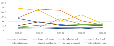
Year	formal rural male	formal rural female	formal urban male	formal urban female	informal rural male	informal rural female	informal urban male	informal urban female
2017-18	131.6	141.4	33.7	243.2	36.5	40.4	26.5	56.3
2018-19	1256.6	1256.6	1265.7	1266.0	682.2	189.4	191.5	199.0
2019-20	90.4	234.1	40.3	217.8	41.6	59.0	29.5	96.6
2020-21	66.77	220.32	129.94	104.87	32.96	61.87	23.03	56.69
2021-22	50.15	108.17	69.87	172.15	34.72	66.46	20.10	51.96
2022-23	59.38	61.99	63.75	75.99	33.17	67.69	33.54	54.05

Download: Download full-size image

Figure 1. For Self-employed Workers.

Among the regular workers, rural males and females within the formal sector and rural females within the informal sector show relatively high inter-spatial variations in terms of wages (Table 2). Further, evidence in favour of sigma convergence is not evident in each of the categories: rather there is an increasing tendency among the formal sector rural male regular workers’ wages while the informal urban female workers experienced a rise in diversity in wages around the Coronavirus Disease (COVID)-19 years before returning to the pre-crisis level of coefficient of variation in 2022-23. Rural female regular workers both in the formal and informal sector registered relatively much higher variations in their wages and showed a declining trend after having a peak in 2020-21 (Figure 2).

Table 2. Coefficient of Variation of Wages for Regular Workers.

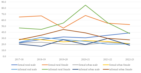
Year	formal rural male	formal rural female	formal urban male	formal urban female	informal rural male	informal rural female	informal urban male	informal urban female
2017-18	22.7	65.2	21.8	28.5	23.3	47.1	20.2	27.6
2018-19	28.0	67.1	23.4	27.5	31.5	44.8	16.8	35.1
2019-20	32.1	46.7	20.0	24.1	27.8	55.1	27.5	44.5
2020-21	30.74	67.66	19.32	26.16	24.92	84.85	19.74	38.88
2021-22	34.95	54.94	23.13	24.67	20.23	55.84	29.64	29.85
2022-23	38.96	52.72	21.18	20.82	20.42	37.78	18.29	27.45

Download: Download full-size image

Figure 2. For Regular Wage Workers.

Among the casual workers again the inter-spatial wage inequality is lower in comparison to the earnings inequality of the self-employed workers. In 2022-23 the informal rural male and female and informal urban female casual workers show higher wage inequality inter-spatially compared to the formal sector workers (Table 3). Over time only among the rural male and female casual workers in the formal sector wage inequality shows a falling tendency. Among the urban female casual workers in the formal sector there was a steady decline between 2017-18 and 2018-19 followed by an increase till 2020-21. Thereafter is again started declining (Figure 3). However, as Figure 3 shows, the wage inequality remained relatively stable over time among many of the categories.

On the whole, inter-spatial wage/earnings inequality is a matter of concern among different types of workers across both the gender and both the regions (rural and urban). These variations do not seem to be disappearing: though in a few instances there is somewhat decline. In the next section we make an attempt to explain these variations in terms of certain important variables.

Table 3. Coefficient of Variation of Wages for Casual Workers.

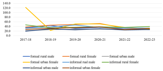
Year	formal rural male	formal rural female	formal urban male	formal urban female	informal rural male	informal rural female	informal urban male	informal urban female
2017-18	34.5	37.5	21.9	122.5	32.5	46.8	19.4	27.2
2018-19	44.1	45.1	25.9	22.9	37.8	34.0	28.8	31.8
2019-20	31.3	48.4	27.8	50.8	46.2	36.5	25.0	34.2
2020-21	35.81	52.55	28.09	50.77	35.04	37.98	29.62	37.37
2021-22	28.48	32.42	26.89	35.48	33.28	35.66	24.55	26.21
2022-23	26.18	27.82	27.79	29.42	32.13	39.26	26.61	31.94

Download: Download full-size image

Figure 3. For Casual Workers.

4. Results from Factor Analysis

Factor analysis technique is followed to reflect on the association among the variables. The number of spatial units being few, we have pooled the time-series and cross-section data. This helps identify significant factors. Then within a given factor the nature of association between different variables and their significance can be examined.

In factor analysis each factor can be said to be a linear combination of a group of variables:

F(j)=Σβ(ij)X(i)+e(j)

j=1…k, and i=1…. n

Where F is the factor, X(i) is the ith variable and β(ij) is the factor loading corresponding to the variable X(i) in the jth factor and e is a random error.

The equation resembles the multiple regression model but they are basic differences between them: the factors are unobservable and we do not have any explicit figure on them while a regression equation the observed values are there on both the dependent and the independent variables.

The factors can be interpreted as hypothetical constructs which can be estimated only from the observed data on the variables. The number of significant factors (k) churned out is usually less than the number of variables, reducing the number of dimensions. Factors with Eigen values or latent roots greater than 1, are considered to be statistically significant 9one rule of thumb) while the Eigen value is computed as the sum of the square of the factor loadings of each of the variables on a given factor. Eigen value is a measure of the amount of variation accounted for by a factor. The proportion of the Eigen value corresponding to a significant factor to the sum of all the Eigen values of all the real factors represents the explained variation in relative terms (a proxy for goodness of fit).

The basic input matrix for factor analysis is the correlation matrix. However, the factor analysis enables us to understand the co-movement of a group of variables in the same and opposite directions. The magnitude of the coefficient of a variable which is otherwise known as factor loadings can vary between 0 and unity (plus or minus). Closer to the modulus value of one would mean that the variable is highly significant and closer to 0 means insignificance. The sign of the coefficient of a variable indicates the nature of its relationship with the other variables. If two variables have positive or negative coefficients, it means a direct relationship between the two. On the other hand, if both have different signs, the co-movement is in the opposite direction.

The results from the rotated factor matrix are analysed because the un-rotated matrix does not ensure that the factors are linearly independent. Since IMR data are not available for all the years, with the inclusion of this variable the number of observations decline significantly. Hence, we have reported the results both with and without IMR.

The wage of the casual workers both in the formal and the informal sector and in the rural and urban areas have relatively high factor loadings, indicating that sectoral and area wise wages are strongly correlated (Table 4). If the formal sector wage is high, so also the informal sector wage and similarly, the rural-urban wage linkages are noticeable. The wage variables are further positively associated with income per capita which is also a proxy for productivity. Though the physical and financial infrastructure variables do not have significant factor loadings, the health specific variable has a significant effect (Table 5), indicating that with improvements in health outcomes wages increase which could be through improvements in the ability to work productively. Since the wages have already been adjusted for price changes the a priori expectation is that the sensitivity of the wages in relation to the price variables may be absent. However, our findings confirm that the prices still generate a positive impact on wages. In other words, in the face of inflation the real wages have a tendency to rise.

Table 4. Results for Casual Workers (with IMR).

Variable	Factor1	Factor2	Factor3
Formal Rural Casual Workers’ Wage	0.5629	0.1322	-0.0365
Formal Urban Casual Workers’ Wage	0.7134	0.2189	-0.1094
Informal Rural Casual Workers’ Wage	0.9199	0.1318	0.1211
Informal Urban Casual Workers’ Wage	0.9470	0.1380	0.0609
NSDP Per Capita	0.4078	-0.0721	0.0822
Per Capita Power	0.1488	-0.1070	-0.0538
Credit-Deposit Ratio	-0.0304	0.0543	-0.3461
Gross Fiscal Deficit	0.1402	0.1601	0.8519
Social Sector Expenditure	-0.0148	-0.0007	0.8721
CPI for Rural Areas	0.1988	0.8972	0.0368
CPI for Urban Areas	0.1621	0.8781	0.1044
IMR	-0.6047	-0.2955	-0.0126

Eigen Value (Proportion Explained in parenthesis): F1=4.27 (0.49), F2=2.03 (0.23), F3=1.50 (0.17); N=114

Source: Authors’ Calculation

Table 5. Results for Casual Workers (without IMR).

Variable	Factor1	Factor2	Factor3
Formal Rural Casual Workers’ Wage	0.5507	0.1148	-0.0558
Formal Urban Casual Workers’ Wage	0.7077	0.2115	-0.0064
Informal Rural Casual Workers’ Wage	0.9161	0.1600	0.1189
Informal Urban Casual Workers’ Wage	0.9258	0.1928	0.0494
NSDP Per Capita	0.4170	-0.0437	0.0650
Per Capita Power	0.1352	-0.0282	-0.0334
Credit-Deposit Ratio	0.0023	0.0753	-0.3716
Gross Fiscal Deficit	0.1379	0.1564	0.8674
Social Sector Expenditure	0.0084	0.1182	0.8945
CPI for Rural Areas	0.1986	0.9233	0.0998
CPI for Urban Areas	0.1659	0.9279	0.1352

Eigen Value (% Explained in parenthesis): F1= 3.83 (0.48), F2=2.06 (0.26), F3=1.32(0.17);

N=169

Source: Authors’ Calculation

Among the regular workers, again the associations across sectors and areas are evident in terms of wage outcomes though the urban formal sector is moderately associated with the rest. Improvements in health indicators and per capita income both raise the wages of the regular workers across sectors and areas (Table 6). The effect of prices on real wages is weakly traceable only in the case of rural areas whereas in the urban areas the sensitivity of the wages of the regular workers to price index is almost absent. As we drop the health indicator the significance of all the wage variables disappears from the factor 1 which is the most significant one (Table 7). Only in factor 3 the informal regular workers’ wages show a positive association, moderate though, across the rural and urban areas. The urban formal sector wages are indicative of a negative association with the informal sector wages and the rural formal sector wages take a negligible factor loading. Power availability and income per capita are positively associated with the informal sector wages. So also, the indicator of financial infrastructure and fiscal deficit though the latter is weakly related. The factor loadings of the price indices are highly negligible.

Table 6. Results for Regular Workers (with IMR).

Variable	Factor1	Factor2	Factor3
Formal Rural Regular Workers’ Wage	0.6857	-0.0740	0.0000
Formal Urban Regular Workers’ Wage	0.3488	-0.1986	-0.0744
Informal Rural Regular Workers’ Wage	0.7780	0.2439	0.0849
Informal Urban Regular Workers’ Wage	0.5669	0.2044	-0.1155
IMR	-0.5873	-0.3721	-0.3559
NSDP Per Capita	0.2512	0.8328	-0.0106
Per Capita Power	0.0352	0.8225	-0.0872
Credit-Deposit Ratio	-0.1711	0.3764	0.0645
Gross Fiscal Deficit	-0.0078	0.1321	0.1992
Social Sector Expenditure	0.0705	-0.1020	-0.0123
CPI for Rural Areas	0.1526	-0.0712	0.9067
CPI for Urban Areas	-0.0736	0.0054	0.8940

Eigen Value (% Explained in parenthesis) = 2.60 (0.35), F2=2.12(0.29), F3 =1.60 (0.22),

N=120

Source: Authors’ Calculation

Table 7. Results for Regular Workers (without IMR).

Variable	Factor1	Factor2	Factor3
Formal Rural Regular Workers’ Wage	0.0198	0.2339	-0.0638
Formal Urban Regular Workers’ Wage	-0.0187	0.0041	-0.2140
Informal Rural Regular Workers’ Wage	0.0240	-0.0066	0.2856
Informal Urban Regular Workers’ Wage	-0.1951	-0.1432	0.2859
NSDP Per Capita	0.0176	0.0620	0.7919
Per Capita Power	0.0099	-0.0352	0.8111
Credit-Deposit Ratio	0.0755	-0.3820	0.3356
Gross Fiscal Deficit	0.1864	0.8611	0.1242
Social Sector Expenditure	0.1187	0.8941	-0.0928
CPI for Rural Areas	0.9411	0.1021	0.0032
CPI for Urban Areas	0.9425	0.1361	0.0151

Eigen Value (% Explained in parenthesis): F1 = 2.36 (0.36), F2=1.96 (0.30), F3=1.59(0.24); N=177

Source: Authors’ Calculation

Among the self-employed workers the earnings are positively associated within the informal sector across the rural and the urban areas. The formal sector earnings are also indicative of a positive correlation between the rural and urban areas though degree of association is rather weak (Table 8 and Table 9). Improvements in infrastructure, overall income/productivity of the region, financial infrastructure and gross fiscal deficit show positive associations with earnings though at varying levels. The sensitivity of the earnings with respect to price is almost absent. These results by and large remain the same with the inclusion of the health indicator: a fall in infant mortality rate is associated with increased earnings.

Table 8. Results for Self-employed Workers (with IMR).

Variable	Factor1	Factor2	Factor3
Formal Rural Self-employed Workers’ Earnings	0.2728	-0.0200	0.0929
Formal Urban Self-Employed Workers’ Earnings	0.2740	-0.0522	-0.1532
Informal Rural Self-employed Workers’ Earnings	0.7960	0.0298	-0.2949
Informal Urban Self-employed Workers’ Earnings	0.8751	-0.1519	0.0881
IMR	-0.4590	-0.4225	-0.0634
NSDP Per Capita	0.8327	0.0699	0.1450
Per Capita Power	0.8475	-0.0226	-0.0451
Credit-Deposit Ratio	0.2957	0.0791	-0.3757
Gross Fiscal Deficit	0.1133	0.1798	0.8581
Social Sector Expenditure	-0.0842	-0.0203	0.8743
CPI for Rural Areas	-0.0350	0.9220	0.0254
CPI for Urban Areas	-0.0449	0.8988	0.0952

Eigen Value (percentage explained in parenthesis): F1=3.35 (0.44), F2=2.16 (0.29), F3=1.62(0.21), N=112

Source: Authors’ Calculation

Table 9. Results for Self-employed Workers (without IMR).

Variable	Factor1	Factor2	Factor3
Formal Rural Self-employed Workers’ Earnings	0.2878	-0.0281	0.1174
Formal Urban Self-Employed Workers’ Earnings	0.2795	0.0329	-0.0055
Informal Rural Self-employed Workers’ Earnings	0.7342	0.0197	-0.2471
Informal Urban Self-employed Workers’ Earnings	0.8822	-0.1331	0.0819
NSDP Per Capita	0.8290	0.0051	0.0508
Per Capita Power	0.7979	0.0383	-0.0440
Credit-Deposit Ratio	0.3227	0.1122	-0.3478
Gross Fiscal Deficit	0.0907	0.1513	0.8659
Social Sector Expenditure	-0.0839	0.0948	0.8929
CPI for Rural Areas	-0.0210	0.9518	0.0628
CPI for Urban Areas	-0.0360	0.9453	0.1283

Eigen Value (% Explained in parenthesis) F1= 3.01 (0.46), F2=2.12 (0.32), F3=1.50 (0.23); N=162

Source: Authors’ Calculation

Minimum Wages and Market Wages/Earnings

With the inclusion of the minimum wage variable a significant number of observations are lost. However, another variable, i.e., industrial productivity on which we do not have observations for all the years can also be considered if minimum wage is included, compromising with the number of observations.

Minimum wages and industrial productivity both show a moderate effect on the wages of the regular workers in the informal sector located in the rural and urban areas both, though the wages of the formal sector regular workers do not seem to get influenced positively (Table 10). Again, on the earnings of the self-employed individuals the minimum wages and industrial productivity show a positive impact, moderately though (Table 11). However, the effect of the minimum wages on the wages of the casual workers is relatively high (Table 12) in comparison to the earnings of the self-employed workers or the wages of the regular workers. Hence, the minimum wage policy can benefit the casual workers who are located at the lowest rungs. Revision of the minimum wage from time to time works as a protection to the workers. It is not just the inter-temporal price change but many other factors which influence the standard of living and wellbeing of the workers need to be considered in setting the minimum wages which are expected to deliver social justice.

Table 10. Results for Regular Workers (with the inclusion of Minimum Wages).

Variable	Factor1	Factor2	Factor3	Factor4
Formal Rural Regular Workers’ Wage	-0.0111	0.2163	0.7306	0.0412
Formal Urban Regular Workers’ Wage	-0.1912	-0.0610	0.4663	-0.0871
Informal Rural Regular Workers’ Wage	0.3137	0.0003	0.6509	0.2443
Informal Urban Regular Workers’ Wage	0.2118	-0.0912	0.4554	0.0448
IMR	-0.3989	0.0065	-0.3979	-0.4806
NSDP Per Capita	0.8455	0.0610	0.1683	0.0664
Per Capita Power	0.9031	-0.0448	-0.0245	-0.1004
Credit-Deposit Ratio	0.3599	-0.3131	-0.2719	-0.0040
Minimum Wages	0.2111	-0.1970	0.0038	0.1203
Gross Fiscal Deficit	0.0948	0.8478	0.0005	0.0980
Social Sector Expenditure	-0.1000	0.8499	0.1097	-0.0131
CPI for Rural Areas	-0.0779	0.0081	0.1756	0.8405
CPI for Urban Areas	-0.0113	0.1125	-0.1146	0.7490
Industrial Productivity	0.3008	0.3606	-0.1140	0.0360

Eigen Values: F1= 2.79, F2=2.44, F3=1.66, F4=1.30; N=88

Source: Authors’ Calculation

Table 11. Results for Self-employed Workers (with the inclusion of Minimum Wages).

Variable	Factor1	Factor2	Factor3
Formal Rural Self-employed Workers’ Earnings	0.2229	0.1852	-0.0936
Formal Urban Self-employed Workers’ Earnings	0.2112	-0.1440	-0.0520
Informal Rural Self-employed Workers’ Earnings	0.8174	-0.2277	0.0644
Informal Urban Self-employed Workers’ Earnings	0.8537	0.1433	-0.0475
Industrial Productivity	0.1825	0.3212	0.0387
IMR	-0.4226	-0.0518	-0.5021
NSDP Per Capita	0.8114	0.1150	0.1378
Per Capita Power	0.8933	-0.0186	-0.0653
Credit-Deposit Ratio	0.2890	-0.2970	-0.0041
Minimum Wages	0.2164	-0.1893	0.1947
Gross Fiscal Deficit	0.1153	0.8613	0.0755
Social Sector Expenditure	-0.0919	0.8380	-0.0100
CPI for Rural Areas	-0.0066	-0.0117	0.8665
CPI for Urban Areas	-0.0297	0.0949	0.7675

Eigen Value: F1=3.73, F2=2.37, F3=1.74; N=82

Source: Authors’ Calculation

Table 12. Results for Casual Workers (with the inclusion of Minimum Wages).

Variable	Factor1	Factor2	Factor3
Formal Rural Casual Workers’ Wage	0.6529	0.3201	-0.1128
Formal Urban Casual Workers’ Wage	0.6984	0.2870	-0.0979
Informal Rural Casual Workers’ Wage	0.9493	0.0778	0.1297
Informal Urban Casual Workers’ Wage	0.9358	0.0977	0.0593
Industrial Productivity	0.1075	0.2148	0.3308
IMR	-0.5796	-0.3823	-0.0072
NSDP per Capita	0.3696	0.7650	0.0750
Per Capita Power	0.1130	0.8949	-0.0406
Credit-Deposit Ratio	-0.0892	0.3200	-0.2904
Minimum Wages	0.4223	0.0479	-0.2083
Gross Fiscal Deficit	0.1258	0.0753	0.8465
Social Sector Expenditure	-0.0182	-0.0822	0.8553
CPI for Rural Areas	0.2457	-0.0638	0.0136
CPI for Urban Areas	0.2336	-0.0882	0.1120

Eigen Value: F1=4.83, F2=2.34, F3=1.64; N=84

Source: Authors’ Calculation

5. Discussion and Policy Implications

Reflecting on the inter-regional wage variations this study explores the role of various factors. If labour is highly mobile, then as per the neoclassical constellation wages are expected to get equalized across space. However, constraints not confined just to the field of economics but also falling into the domain of sociology, culture and geography reduce the pace of population movement and affects the validity of the wage-equalization hypothesis. In fact, the variations in wages and earnings across the Indian states are seen to be significant, and overtime the sigma convergence does not seem to be taking place. This prompted us to investigate the wage issue further. Which factors can help raise the wages so that the areas with lower wages and earnings will be able to catch up with the better off regions even when inter-state migration is not significant?

The factors considered in the study include physical infrastructure, financial infrastructure, health, growth and productivity indicator, prices, policy variable such as minimum wage set by the state governments, fiscal deficit and social expenditure incurred by the government. Factor analysis results show that physical infrastructure, financial infrastructure, health, growth, and productivity indicators have a significant relationship with real wages/earnings which is indicative of the fact that many variables impact the wages/earnings across states and union territories. Findings are indicative of the fact that wages and earnings respond to the infrastructure and health related indicators. Economic growth and productivity rise also show a positive impact. Besides, the minimum wage policy of the government is seen to be effective. Though the real wages have been calculated after making the adjustments for price changes, their responsiveness to the consumer price index is not absent altogether.

We are also able to see linkages between the formal sector wages/earnings and the informal sector wages/earnings. Encouraging formal sector jobs in states or encouraging private investment can affect the wages/earnings in the informal sector across rural and urban spaces. The fact that the labour markers across regions and sectors are actually inter-connected, and not independent of each other, bear a great deal of insight into our understanding of the urban and labour economics literature.

It is important for governments to prioritize policies that promote economic development in lagging states. Infrastructure investments, encouraging industries to set up in less-developed regions, and supporting skill development can all be included. Creating a framework for a national minimum wage is also a viable option for policymakers to reduce extreme disparities, but it is necessary to take into account the regional cost-of-living differences. Also, the focus on employment generation programs like the Mahatma Gandhi National Rural Employment Guarantee Act (MGNERA) can be targeted toward states with low wages to raise income levels.

Policymakers may have to consider these macro-economic variables for different spaces before reaching into any decision related to wages/earnings. These macro-economic variables can also facilitate population mobility which in turn would contribute to equalization of wages/earning across space.

Abbreviations

OECD	Organization for Economic Co-operation and Development
NSDP	Net State Domestic Product
CPI	Consumer Price Index
IMR	Infant Mortality Rate
MoSPI	Ministry of Statistics and Programme Implementation
CEA	Central Electricity Authority
CDR	Credit-deposit Ratio
GFD	Gross Fiscal Deficit
RBI	Reserve Bank of India
NSO	National Statistics Office
ASI	Annual Survey of Industries
COVID	Coronavirus Disease

Conflicts of Interest

The authors declare no conflicts of interest.

References

[1]	Ahluwalia, Rahul, Rana Hasan, Mudit Kapoor and Arvind Panagariya (2018), The Impact of Labor Regulations on Jobs and Wages in India: Evidence from a Natural Experiment, Working Paper No. 2018-02, Columbia, SIPA, Deepak and Neera Raj Centre on Indian Economic Policies.
[2]	Autor, D. (2015) Why Are There Still So Many Jobs? The History and Future of Workplace Automation, Journal of Economic Perspectives 29(3): 3-30.
[3]	Banerjee, Abhijit V. and Esther Duflo and Duflo (2014). Do Firms Want to Borrow More? Testing Credit Constraints Using a Directed Lending Program, The Review of Economic Studies, Volume 81, Issue 2, April 2014, Pages 572–607.
[4]	Djidonou, Gbenoukpo Robert and Neil Foster-McGregor, (2020), Stagnant manufacturing growth in India: The role of the informal economy, Maastricht Economic and social Research institute on Innovation and Technology (UNU-MERIT) website: http://www.merit.unu.edu Boschstraat 24, 6211 AX Maastricht, The Netherlands.
[5]	Faozi A. Almaqtari & Najib H. S. Farhan & Ali T. Yahya & Eissa A. Al-Homaidi, 2020. "Macro and socio-economic determinants of firms' financial performance: empirical evidence from Indian states," International Journal of Business Excellence, Inderscience Enterprises Ltd, vol. 21(4), pages 488-512.
[6]	Jain, Hansa (2019), Wage–Productivity Relationship in Indian Manufacturing Industries: Evidence from State-level Panel Data, Margin The Journal of Applied Economic Research 13(3): 277-305, https://doi.org/10.1177/0973801019841258
[7]	Korinek, Anton and Joseph E. Stiglitz, (2017), Artificial Intelligence and Its Implications for Income Distribution and Unemployment, NBER Working Paper Series, Working Paper 24174 http://www.nber.org/papers/w24174
[8]	Kumar, U and P Mishra (2008): “Trade Liberalisation and Wage Inequality: Evidence from India,” Review of Development Economics, Vol 12, No 2, pp 291–311.
[9]	Mills, E. S. (1999), "Earnings inequality and central-city development," Economic Policy Review, Federal Reserve Bank of New York, vol. 5(Sep), pages 133-142.
[10]	Mills, E. S. (1967), An Aggregative Model of Resource Allocation in a Metropolitan Area, The American Economic Review, Vol. 57, No. 2, Papers and Proceedings of the Seventy-ninth Annual Meeting of the American Economic Association (May, 1967), pp. 197-210.
[11]	Mitra, Arup (2023), Barriers to Employment: Impact of Macro, Individual and Enterprise-level Variables (SpringerBriefs in Economics) Paperback – Import, 5 August 2023.
[12]	Mitra, Arup & Varoudakis, Aristomene & Veganzones-Varoudakis, Marie-Ange, 2002. "Productivity and Technical Efficiency in Indian States' Manufacturing: The Role of Infrastructure," Economic Development and Cultural Change, University of Chicago Press, vol. 50(2), pages 395-426, January.
[13]	OECD, 2007, Economic Policy Reforms: Going for Growth, https://www.oecd.org/economy/growth/economicpolicyreformsgoingforgrowth2007.htm
[14]	Szirmai, Adam (2012) Industrialisation as an engine of growth in developing countries, 1950–2005, Structural Change and Economic Dynamics, vol. 23, issue 4, 406-420.
[15]	Ugur, M and Arup Mitra (2017) Technology Adoption and Employment in Less Developed Countries: A Mixed-Method Systematic Review, World Development, vol. 96, issue C, 1-18.

Cite This Article

Plain Text BibTeX RIS

APA Style

Mitra, A., Mishra, S. (2025). Wages Across Regions: Responsiveness to Macro and Policy Variables. Journal of World Economic Research, 14(1), 13-25. https://doi.org/10.11648/j.jwer.20251401.12

Copy | Download

ACS Style

Mitra, A.; Mishra, S. Wages Across Regions: Responsiveness to Macro and Policy Variables. J. World Econ. Res. 2025, 14(1), 13-25. doi: 10.11648/j.jwer.20251401.12

Copy | Download

AMA Style

Mitra A, Mishra S. Wages Across Regions: Responsiveness to Macro and Policy Variables. J World Econ Res. 2025;14(1):13-25. doi: 10.11648/j.jwer.20251401.12

Copy | Download

@article{10.11648/j.jwer.20251401.12,
  author = {Arup Mitra and Sarthak Mishra},
  title = {Wages Across Regions: Responsiveness to Macro and Policy Variables
},
  journal = {Journal of World Economic Research},
  volume = {14},
  number = {1},
  pages = {13-25},
  doi = {10.11648/j.jwer.20251401.12},
  url = {https://doi.org/10.11648/j.jwer.20251401.12},
  eprint = {https://article.sciencepublishinggroup.com/pdf/10.11648.j.jwer.20251401.12},
  abstract = {This study reflects on the inter-regional wage variations. If labour is highly mobile then as per the neoclassical constellation wages are expected to get equalized across space. But the variations in wages and earnings across the Indian states are seen to be significant. This prompted us to investigate the wage variation issue further. The factors considered in the study include physical infrastructure, financial infrastructure, health, growth indicator, prices, policy variable such as minimum wage set by the state governments and the fiscal deficit, which may impact on wages across space. Findings are indicative of the fact that wages and earnings respond to the infrastructure and health related indicators. Economic growth and productivity rise also show a positive impact. Besides, the minimum wage policy of the government is seen to be effective, particularly in the case of those who are located at the lower rungs. The real wages/earnings do not show any significant responsiveness to price index though the association is not totally absent. Finally, the policy implications of the study are brought out.
},
 year = {2025}
}

Copy | Download

TY - JOUR
T1 - Wages Across Regions: Responsiveness to Macro and Policy Variables

AU - Arup Mitra
AU - Sarthak Mishra
Y1 - 2025/01/24
PY - 2025
N1 - https://doi.org/10.11648/j.jwer.20251401.12
DO - 10.11648/j.jwer.20251401.12
T2 - Journal of World Economic Research
JF - Journal of World Economic Research
JO - Journal of World Economic Research
SP - 13
EP - 25
PB - Science Publishing Group
SN - 2328-7748
UR - https://doi.org/10.11648/j.jwer.20251401.12
AB - This study reflects on the inter-regional wage variations. If labour is highly mobile then as per the neoclassical constellation wages are expected to get equalized across space. But the variations in wages and earnings across the Indian states are seen to be significant. This prompted us to investigate the wage variation issue further. The factors considered in the study include physical infrastructure, financial infrastructure, health, growth indicator, prices, policy variable such as minimum wage set by the state governments and the fiscal deficit, which may impact on wages across space. Findings are indicative of the fact that wages and earnings respond to the infrastructure and health related indicators. Economic growth and productivity rise also show a positive impact. Besides, the minimum wage policy of the government is seen to be effective, particularly in the case of those who are located at the lower rungs. The real wages/earnings do not show any significant responsiveness to price index though the association is not totally absent. Finally, the policy implications of the study are brought out.

VL - 14
IS - 1
ER -

Copy | Download

Author Information

Arup Mitra

Faculty of Economics, South Asian University, New Delhi, India

Contact Email

http://orcid.org/0000-0002-9386-1402
Sarthak Mishra

Department of Economics, Delhi School of Economics, Delhi, India

Contact Email

Download PDF

Plain Text BibTeX RIS

APA Style

Mitra, A., Mishra, S. (2025). Wages Across Regions: Responsiveness to Macro and Policy Variables. Journal of World Economic Research, 14(1), 13-25. https://doi.org/10.11648/j.jwer.20251401.12

Copy | Download

ACS Style

Mitra, A.; Mishra, S. Wages Across Regions: Responsiveness to Macro and Policy Variables. J. World Econ. Res. 2025, 14(1), 13-25. doi: 10.11648/j.jwer.20251401.12

Copy | Download

AMA Style

Mitra A, Mishra S. Wages Across Regions: Responsiveness to Macro and Policy Variables. J World Econ Res. 2025;14(1):13-25. doi: 10.11648/j.jwer.20251401.12

Copy | Download

@article{10.11648/j.jwer.20251401.12,
  author = {Arup Mitra and Sarthak Mishra},
  title = {Wages Across Regions: Responsiveness to Macro and Policy Variables
},
  journal = {Journal of World Economic Research},
  volume = {14},
  number = {1},
  pages = {13-25},
  doi = {10.11648/j.jwer.20251401.12},
  url = {https://doi.org/10.11648/j.jwer.20251401.12},
  eprint = {https://article.sciencepublishinggroup.com/pdf/10.11648.j.jwer.20251401.12},
  abstract = {This study reflects on the inter-regional wage variations. If labour is highly mobile then as per the neoclassical constellation wages are expected to get equalized across space. But the variations in wages and earnings across the Indian states are seen to be significant. This prompted us to investigate the wage variation issue further. The factors considered in the study include physical infrastructure, financial infrastructure, health, growth indicator, prices, policy variable such as minimum wage set by the state governments and the fiscal deficit, which may impact on wages across space. Findings are indicative of the fact that wages and earnings respond to the infrastructure and health related indicators. Economic growth and productivity rise also show a positive impact. Besides, the minimum wage policy of the government is seen to be effective, particularly in the case of those who are located at the lower rungs. The real wages/earnings do not show any significant responsiveness to price index though the association is not totally absent. Finally, the policy implications of the study are brought out.
},
 year = {2025}
}

Copy | Download

TY - JOUR
T1 - Wages Across Regions: Responsiveness to Macro and Policy Variables

VL - 14
IS - 1
ER -

Copy | Download