Comparative Analysis of ARIMA, SARIMA and Prophet Model in Forecasting

Samuel Baffoe Kwarteng; Poguda Aleksey Andreevich

doi:doi:10.11648/j.rd.20240504.13

Research Article |

| Peer-Reviewed

Comparative Analysis of ARIMA, SARIMA and Prophet Model in Forecasting

Samuel Baffoe Kwarteng^*

, Poguda Aleksey Andreevich

Published in Research & Development (Volume 5, Issue 4)

Received: 7 September 2024 Accepted: 24 September 2024 Published: 18 October 2024

Views: Downloads:

Download PDF

Share This Article

Twitter
Linked In
Facebook

Abstract

Machine learning has become a powerful tool in forecasting, offering greater accuracy than traditional human predictions in today’s data-driven world. The capability of machine learning to predict future trends has significant implications for key sectors such as finance, healthcare, and supply chain management. In this study, ARIMA/SARIMA (AutoRegressive Integrated Moving Average/Seasonal AutoRegressive Integrated Moving Average), alongside Prophet, a scalable forecasting tool developed by Facebook based on a generalized additive model, are considered. These models are applied to predict the demand for antidiabetic drugs. The records were collected by the Australian Health Insurance Commission. This dataset was sourced from Medicare Australia. The study evaluates the performance of these models based on their Mean Absolute Error (MAE), a key metric for assessing forecast accuracy. Root Mean Squared Error (RMSE) and Mean Absolute Percentage Error (MAPE) are also considered. The outcome of the comparative analysis shows that the Prophet model outperformed both ARIMA and SARIMA models, achieving an MAE of 0.74, which is significantly lower than the MAE values of 2.18 and 3.02 obtained by SARIMA and ARIMA, respectively. Prophet's superior performance shows its effectiveness in handling complex, non-linear trends and seasonal patterns often observed in real-world time series data. This research contributes to the growing knowledge of machine learning-based forecasting and shows the importance of advanced models like Prophet in optimizing business operations and driving innovation. The findings from this research offer valuable guidance for data experts, analysts, and researchers in selecting the best forecasting methods for reliable predictions.

Published in	Research & Development (Volume 5, Issue 4)
DOI	10.11648/j.rd.20240504.13
Page(s)	110-120
Creative Commons	This is an Open Access article, distributed under the terms of the Creative Commons Attribution 4.0 International License (http://creativecommons.org/licenses/by/4.0/), which permits unrestricted use, distribution and reproduction in any medium or format, provided the original work is properly cited.
Copyright	Copyright © The Author(s), 2024. Published by Science Publishing Group

Keywords

AutoRegressive Integrated Moving Average (ARIMA), Seasonal AutoRegressive Integrated Moving Average (SARIMA), Mean Absolute Percentage Error (MAPE), Prophet, Time Series Forecasting, Comparative Analysis

1. Introduction

In today's world, where we use data to make important decisions, it is important for businesses, researchers, and analysts in different fields to be able to predict what might happen in the future. One type of data that is super useful for this is time series data. Time Series analysis assumes that future demand will be similar to past demand and involves analyzing historical data to make predictions. Techniques used in time-series analysis include trend analysis, seasonal analysis, and moving averages. A study by Bharatpur, A., et al. discusses the observation of a growing or decreasing pattern over time, known as a trend

[1]

. In contrast to conventional time series, where the mean can vary at will with respect to time, stationary time series require that the data's mean remain constant across time. Seasonality is the term for a cycle of events. A pattern, after some time, keeps happening. Seasonality can be influenced by factors like holidays, weather changes, or business cycles. This paper builds upon existing research in this area, focusing on the task of predicting antidiabetic drugs in Australia. It aims to compare the effectiveness of two prominent time series forecasting models: AutoRegressive Integrated Moving Average (ARIMA/SARIMA) and the Facebook Prophet model. The ARIMA model, developed by Box and Jenkins in 1976, is used to analyze stationary univariate time series data. SARIMA models are an extension of the ARIMA model designed to handle seasonal or cyclic components in time series data.

ARIMA/SARIMA models can model the linear and seasonal dependencies in the data, while the Facebook Prophet model is a novel approach that can handle multiple seasonalities, holidays, and other factors using a decomposable time series model. What sets Prophet apart is its ability to automatically detect and accommodate various seasonal patterns, as well as adjust for the effects of holidays and special events. Moreover, it offers flexibility in incorporating prior knowledge and domain expertise through user-specified parameters and regressors.

In contrast to the intricate tuning requirements of traditional ARIMA models, the paper by Taylor, S., et al. highlighted the limitations of traditional models like ARIMA in terms of complexity and the need for expertise in tuning parameters

[2]

. The paper also provides a comparison of the Prophet model with other popular forecasting methods, such as exponential smoothing, ARIMA, and structural time series models. The authors claim that the Prophet model is more flexible, scalable, and interpretable than the existing methods, and that it can produce high quality forecasts for a wide range of business problems.

A study by Yenidogan, I., et al. compared two methods, PROPHET and ARIMA, for forecasting Bitcoin prices using data from May 2016 to March 2018

[3]

. Additional variables were included in the models based on correlation studies between cryptocurrencies and real currencies to improve forecasting accuracy. PROPHET performed better than ARIMA, with R² values of 0.94 and 0.68, respectively. PROPHET had a prediction accuracy of 94.5%, which was higher than ARIMA. The study recommends using PROPHET for Bitcoin forecasting because it gives more accurate predictions compared to ARIMA, which had a lower precision rate of 68%. However, SARIMA can be used in conjunction with other techniques to enhance forecasting accuracy. The authors of the document in

[4]

proposed a hybrid model that combines SARIMA with artificial neural networks (ANNs) and fuzzy logic to address the limitations of SARIMA models in time series forecasting tasks.

The findings of F. V. Ferdinand et al.

[5]

showed that SARIMA demonstrated superior performance in their research due to its emphasis on testing for stationarity and hyperparameter tuning. This study illustrates the critical importance of model selection.

In a separate study by Wang et al.

[6]

, the authors proposed the ARIMA, SARIMA, and Prophet models to predict daily new cases and cumulative confirmed cases of COVID-19 in the USA, Brazil, and India over a 30-day period. Their results indicated that for the USA, the SARIMA model had limitations and ranked as the second-best option. In contrast, for Brazil and India, the ARIMA model was second-best after the Prophet model for daily new cases. This shows that selecting a forecasting model requires careful consideration of the specific needs of each task, as the Prophet model does not always guarantee the best results.

This paper is structured as follows: The description of the dataset and preprocessing is discussed in Section II. Section III talks about the development of the ARIMA and SARIMA models, finding the optimal order, and the Prophet model for making predictions. The experimental results are analyzed in Section IV, whereas conclusions are drawn in Section V.

2. Materials and Methods

2.1. Description of Dataset and Preprocessing

A dataset (Figure 1) containing a number of anti-diabetic drug prescriptions in Australia was used. The records were collected by the Australian Health Insurance Commission from year 1991 to 2008. This dataset was sourced from Medicare Australia. In Australia, Medicare serves as the country's publicly funded universal healthcare insurance system. It is operated by Australia's social security department, which works in conjunction with the Pharmaceutical Benefits Scheme.

Download: Download full-size image

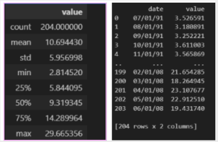
Figure 1. Shape and Description of Dataset.

Data preprocessing is imperative to ensure the accuracy of results. Training data can be with errors and outliers which can significantly impact the final model's efficacy. Data cleaning involves the identification and removal of attributes with insufficient data or those lacking variance. These data points, both rows and columns, must be dropped from the training dataset. Python provides powerful tools for this task, such as the isnull () function from the pandas library to check for missing data and the dropna () function to eliminate rows or columns containing missing values.

Changes that happen regularly during seasons are usually the most important part of a seasonal time series; an example is the "stochastic trend" - sometimes comes along with the seasonal patterns. This trend can actually affect how well different methods for prediction work. Figure 2 displays a noticeable trend over time, it is typically not in a stable state and requires adjustments before it can be used for making predictions. Being able to predict accurately in time series data that has both trends and seasonal patterns is important because it helps make good decisions in many different areas.

Download: Download full-size image

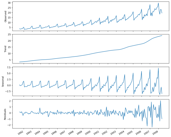
Figure 2. The decomposition of the monthly number of antidiabetic drug prescriptions in Australia between 1991 and 2008. The first plot illustrates the observed data. The second plot demonstrates the trend component, which exhibits a consistent increase over time. The third plot shows the seasonal component, which is distinctly observed as recurring through time. Finally, the last plot represents the residuals, which signify the variations in the data that cannot be explained by the trend or the seasonal component.

2.2. Time Stationary Identification

In time series analysis, the identification of stationarity is essential as the analysis relies solely on stationary data. Christophorus et al. emphasized the need to check whether the time series is stationary

[7]

. The Augmented Dickey-Fuller (ADF) test emerges as a widely used statistical tool for this purpose. When the test statistic falls below the critical value, the null hypothesis is rejected, indicating stationarity within the series. Conversely, if the test statistic exceeds the critical value, failing to reject the null hypothesis suggests non-stationarity. The outcomes of the ADF test are summarized in Table 1.

Table 1. Result of ADF Test for antidiabetic drug prescriptions.

	Value
ADF Statistics	3.145185689306735
p- value	1.0
Number of Lags Used	15
Number of Observations	188
Critical Values	1%: -3.465620397124192 5%: -2.8770397560752436 10%: -2.5750324547306476

In Figure 3, to address nonstationary within the series, a differencing technique was used. Initially, the `np.diff()` function was used with a lag of 1 (n=1), effectively reducing trends and seasonality, thus rendering the series more stationary. Following this initial differencing step, a further seasonal differencing was performed using a lag of 12 (n=12) to account for seasonal patterns. Subsequently, a second iteration of the Augmented Dickey-Fuller (ADF) test was conducted on the seasonally differenced series (`y_diff_seasonal_diff`) to confirm the effectiveness of the differencing technique in achieving stationarity. The assessment of the ADF statistic and its associated p-value provided a comprehensive evaluation of the stationarity characteristics of the seasonally differenced series. This additional analysis further validated the efficacy of the differencing technique in enhancing the stationarity of the series.

Download: Download full-size image

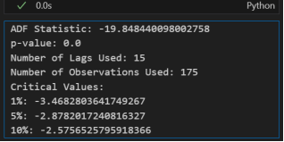
Figure 3. Augmented Dickey-Fuller Test.

3. Arima and Sarima Model Development

3.1. AutoRegressive Integrated Moving Average Model

An autoregressive integrated moving average process combines an autoregressive process (AR(p)), integration (I(d)), and a moving average process (MA(q)). Peixeiro stated that parameter selection (p, d, q) can be challenging, but it offers interpretability through linear combinations of past values and errors. However, handling seasonality may necessitate additional adjustments.

[8].

Ali Hussein et al. stated that in a non-seasonal ARIMA (p, d, q) model, the number or order of AR terms is denoted by p, the number or order of differences by d, and the number or order of MA terms by q

[9]

Auto regressive Series, In Equation 1

Y_{t}

is called an autoregressive series of order

p

AR (p)

if it satisfies

Y_{t} = ∳_{1} Y_{t - 1} + \dots + ∳_{p} Y_{t - p} + ε_{t}

(1)

where is

ε_{t}

white noise and the

∳_{u}

are parameter coefficients. The next value observed in the series is a slight perturbation of a simple function of the most recent observations. The Moving Average from Equation 2

Y_{t}

is called a moving average process of order

q

MA (q)

if it satisfies

Y_{t} = ε_{t} + θ_{1} ε_{t - 1} + \dots + θ_{q} ε_{t - q}

(2)

where

θ_{u}

are parameters coefficients. When working on a time series model it is quite easier to spot the difference between MA and AR series by using their Auto Correlation Functions (ACF), MA ACF cuts off sharply while AR ACF decays exponentially.

Integrated Series has the value of

Y_{t}

being the sum of the random values. The order of integration d is the number of differencings a series requires to be made stationary. A random walk process is an example of I(d).

For the purposes of model training and evaluation, the dataset was divided into two distinct subsets: the training set and the test set. The training set, comprising the first 168 observations of the time series data, was used to train the predictive model. This segment of the data was selected to provide an adequate historical context for the model to learn patterns and trends. The test set comprises the data that was not used for training, specifically the observations from index 168 onwards. Its purpose is to evaluate the model's performance. By holding back this data during training, a fair assessment of the model's predictions is ensured because it has not encountered this data previously. This approach enables an accurate gauge of the model’s effectiveness.

Download: Download full-size image

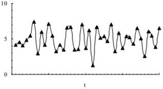
Figure 4. An example of MA(1) process, produced using a number generator.

Download: Download full-size image

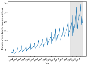
Figure 5. Train set and test split for antidiabetic drug dataset. The shaded area is the testing period.

A list of all possible combinations of the parameters p, q, P, and Q is generated using the product function from the itertools module, creating the ARIMA_order_list. The parameters of the final model are determined by finding the combination with the lowest AIC value, which is 347.946664. The ARIMA model is created using the SARIMAX function, utilizing the training dataset and configured with an order of (12,2,10). The model is then fitted to the training data using the fit method. To assess whether the residuals of the model conform to a normal distribution, the Ljung-Box test is used, this produces a p-value of 0. Hence, the original hypothesis (H0: residuals are normally distributed) cannot be rejected. The residuals are analyzed by plotting ACF plots, Q-Q plots, and histograms (Figure 6).

Download: Download full-size image

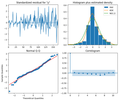
Figure 6. ARIMA diagnostic plot.

3.2. Seasonal AutoRegressive Integrated Moving Average Model

The SARIMA(p,d,q)(P,D,Q)m model expands on the ARIMA(p,d,q) model by adding seasonal parameters. The parameters in the model P, D, Q, and m. (p,d,q) correspond to their seasonal counterparts, augmenting the model's capability to handle seasonal variations.

1) p,d,q: These parameters have the same meanings as in the ARIMA(p,d,q) model, representing the autoregressive, differencing, and moving average component and moving respectively.

2) P: It represents the order of the seasonal autoregressive (AR) process, indicating the lagged values in the seasonal component.

3) D: This parameter denotes the seasonal order of integration, similar to d but applied to the seasonal component.

4) Q: It denotes the order of the seasonal moving average (MA) process, capturing the lagged error terms in the seasonal component.

5) m: This parameter represents the frequency, indicating the number of observations per seasonal cycle. The length of the cycle depends on the dataset and the nature of the seasonality present.

SARIMA(p,d,q)(P,D,Q)m model allows for a comprehensive modeling of both non-seasonal and seasonal components in time series data, providing a powerful framework for forecasting and analysis.

The model has a non-seasonal order of (3,1,3) and a seasonal order of (3,1,3,12), which means it considers seasonal patterns every 12 time periods. The model results in Table 2 indicate the following:

Table 2. SARIMA model results.

Dependent variable	Values
Total number of observations used in the analysis	169
Model specifications	SARIMAX(3, 1, 3)x(3, 1, 3, 12), indicating a seasonal and non-seasonal order of (3, 1, 3) and (3, 1, 3, 12) respectively
log likelihood of the model	-125.920
Akaike Information Criterion (AIC)	277.841
Bayesian Information Criterion (BIC)	317.489
Hannan-Quinn Information Criterion (HQIC)	293.944

Figure 7 shows two forecast models for the drug distribution: the ARIMA(12,2,10) model and the SARIMA(3,1,3)(3,1,3,12) model. The blue line is the actual distribution over time, giving a basis for checking the accuracy of the models. The black dashed line is from the ARIMA(12,2,10) model, and the green dash-dotted line is from the SARIMA(3,1,3)(3,1,3,12) model. Comparing the model predictions to the actual distribution, both models capture some trends and patterns, but their accuracy and ability to catch all the details might differ. The shaded area marks the period of comparison (from index 168 onwards), helping focus on how well the models perform during this time.

Download: Download full-size image

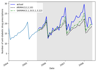
Figure 7. Actual and Predicted Drug Distribution using ARIMA and SARIMA Models.

3.3. Prophet Model

Prophet is ideal for time series data with strong and multiple seasonal patterns. It can detect daily, weekly, and yearly seasonality, including holidays and special events. Prophet is user-friendly, requiring minimal data preprocessing, and offers uncertainty estimation via prediction intervals. The package is available for use with Python. It allows you forecast rapidly with minimal manual work.

These factors include y(t) which is modeled as the linear combination of:

1) a trend g(t);

2) a seasonal component s(t);

3) holiday effects h(t);

4) an error term ϵt, which is normally distributed.

Mathematically, this can be expressed as:

y (t) = g (t) + s (t) + h (t) + ϵt,

(3)

where g(t) is the trend; s(t) is the seasonal component; h(t) is the holiday effects; ϵt is the error term. The g(t) component, representing the trend, is accountable for the non-periodic long-term changes observed in the time series. On the other hand, the seasonal component (s(t)) captures the periodic changes, whether they occur yearly, monthly, weekly, or daily. In real-time scenarios, holidays play a significant role in our daily lives, making the h(t) component crucial in the functioning of the model. Holiday effects tend to occur irregularly and may span over multiple days. In cases where there is a deviation in values that cannot be explained by any of the three aforementioned components, the error term ϵt is responsible for it.

To account for multiple seasonal periods, Prophet employs Fourier series to model these periodic effects. Human behaviors often generate time series data with multiple periodicities. For instance, the typical five-day workweek can produce a pattern that repeats weekly, while school breaks may generate a pattern recurring annually.

s (t) = \sum_{n = 1}^{N} (a_{n} \cos \cos (\frac{2 πnt}{P}) + b_{n} \sin \sin (\frac{2 πnt}{P}),

(4)

where s(t) the seasonal component; P is the length of the seasonal period in days; N is the number of terms in the Fourier series. In Russia, on December 31st, there is typically a notable surge in store attendance or e-commerce sales. Prophet provides an alternative solution, by allowing users to define a list of holidays for a specific country. Prophet utilizes 10 terms to model the yearly seasonality and 3 terms to model the weekly seasonality. If a data point falls on a holiday date, a parameter Ki is calculated to represent the change in the time series at that point in time. The magnitude of this change correlates with the holiday effect: the larger the change, the more pronounced the holiday effect.

Figure 8 shows the actual antidiabetic drug sales as black dots, the forecasted sales as a blue line, and the uncertainty intervals as a shaded blue area. Future time periods are forecasted accordingly.

Download: Download full-size image

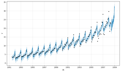
Figure 8. Forecasted Antidiabetic Drug Sales.

The plotted graph in Figure 9 shows the comparison between actual and predicted drug distribution over time. The blue line represents the actual distribution data, while the red line depicts the predicted distribution based on the forecast model. As shown in the graph, the model's predictions align closely with the actual distribution trends, indicating the effectiveness of the forecasting approach.

Download: Download full-size image

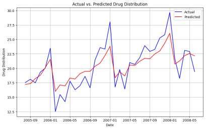
Figure 9. Actual vs. Predicted Drug Distribution.

Table 3 shows the forecast with key columns: future dates ('ds'), forecasted values ('yhat'), and their lower ('yhat_lower') and upper ('yhat_upper') bounds considering uncertainty.

Table 3. Forecasted Values.

	ds	yhat	yhat_lower	yhat_upper
201	2008-04-01	22.195313	20.914156	23.543719
202	2008-05-01	22.575389	21.302224	23.803814
203	2008-06-01	22.148415	20.802760	23.391756
204	2008-06-02	21.477172	20.162868	22.749761
205	2008-06-03	20.848034	19.475679	22.144559
206	2008-06-04	20.272289	18.942728	21.561791
207	2008-06-05	19.759586	18.391037	21.124836
208	2008-06-06	19.317742	18.003627	20.687164
209	2008-06-07	18.952615	17.711169	20.339748
210	2008-06-08	18.668027	17.366279	20.009852

4. Results

Download: Download full-size image

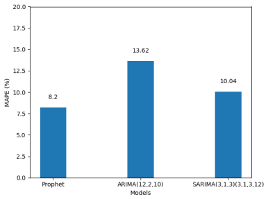
Figure 10. MAPE Evaluation.

The outcomes of the models were analyzed with a specific emphasis on the evaluation of performance metrics. Specifically, the evaluation will use three key metrics: Mean Absolute Error (MAE), Root Mean Squared Error (RMSE), and Mean Absolute Percentage Error (MAPE). These metrics provide valuable insights into the accuracy and reliability of each model’s predictions. While MAPE is commonly used in forecasting studies, recent research has shown limitations associated with RMSE. Botchkarev, A. cautioned against relying solely on RMSE due to its 'disturbing characteristics', suggested instead the use of MAE as a more appropriate error measure

[10]

. Additionally, Vogt, M. R. et al. proposed a composite metric that combines several statistical indices, including CV(RMSE), NME, and contingency coefficients, as a comprehensive performance measure for dynamic simulations

[11]

The results and MAPE of each model are presented in Figure 10. The MAPE values are represented on the y-axis, while the models are listed on the x-axis. For Prophet, the MAPE is 8.2%, while for ARIMA(12,2,10) and SARIMA(3,1,3)(3,1,3,12), the MAPE values are 13.62% and 10.04%, respectively. The chart provides a visual comparison of the forecast error among these models.

Experimental Analysis shows that the PROPHET model performs better than the ARIMA and SARIMA models. This is evident when predicting the next 10 days from July 1, 2008. The results in Table 4 display the predicted values. On July 1, 2008, the ARIMA model forecasted a value of 18.868517, the SARIMA model predicted 20.666992, and the PROPHET model forecasted 23.495457.

Table 4. Comparison of the three models.

	ds	ARIMA_predictions	SARIMA predictions	PROPHET predictions (yhat)
233	2008-07-01	18.868517	20.666992	23.495457
234	2008-07-02	19.079705	20.665763	23.615460
235	2008-07-03	20.342761	21.313098	23.716462
236	2008-07-04	19.584552	22.557885	23.802352
237	2008-07-05	21.170749	22.786816	23.877175
238	2008-07-06	21.869748	24.273169	23.944934
239	2008-07-07	23.048193	27.043418	24.009401
240	2008-07-08	16.434465	17.595999	24.073943
241	2008-07-09	16.791910	19.208757	24.141377
242	2008-07-10	18.201320	19.747515	24.213838

While MAE treats all errors equally, RMSE solves problem with larger errors more heavily due to the squaring of differences.

[4]

MAE proves less sensitive to outliers, making it a perfect choice for assessing model accuracy. In Figure 11, the Prophet Model achieves a lower MAE value as compared to ARIMA and SARIMA.

Download: Download full-size image

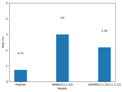
Figure 11. MAE Evaluation.

A lower MAE value signifies improved model performance, indicating predictions that closely align with actual values.

[12]

Download: Download full-size image

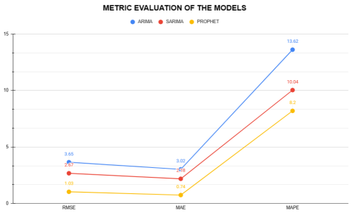
Figure 12. Metric Evaluation of the Models.

The evaluation of performance metrics offer valuable insights into different aspects of model performance, such as the magnitude of errors, the impact of outliers, and the overall forecast accuracy.

5. Discussion

This study compared two powerful time series models, the AutoRegressive Integrated Moving Average (ARIMA) model, the Seasonal AutoRegressive Integrated Moving Average (SARIMA) model, and the Prophet model, in the context of forecasting antidiabetic drug sales in Australia. The dataset exhibited seasonality, making it essential to use models capable of capturing seasonal components for accurate predictions.

The experimental setup involved training the models on the initial 168 observations of the dataset, with the test set comprising data from index 168 onwards. After the model training and testing phases, the results were analyzed and errors were recorded to evaluate the performance of the model.

Three key metrics, Mean Absolute Error (MAE), Root Mean Squared Error (RMSE), and Mean Absolute Percentage Error (MAPE), were used to assess the accuracy and precision of the models' predictions. The findings revealed that the Prophet model exhibited superior performance by recording lower error values compared to both the ARIMA and SARIMA models.

In the evaluation of the models, the SARIMA model emerged as the second-best performer, surpassing the ARIMA model. The SARIMA model's ability to capture seasonal components and provide sophisticated modeling of time series data contributed to its enhanced predictive capabilities. This observation proves that SARIMA models excel in handling datasets with pronounced seasonality, and finding complex temporal patterns in data. The univariate nature of the dataset aligned well with the modeling strengths of ARIMA, which typically performs better on univariate data.

6. Conclusion

The superior performance of the Prophet model across three evaluation metrics shows the effectiveness of the Prophet model in handling time series forecasting tasks. The combination of advanced modeling techniques, automatic seasonal pattern detection, flexibility, scalability, uncertainty estimation, and user-friendly interface makes Prophet the best model amongst ARIMA and SARIMA in the study.

Future research could explore the application of neural networks, extreme gradient boosting, as demonstrated by Nain et al.

[13]

, Long term short- term algorithm, alongside the Prophet model to enhance accuracy and adaptability under various conditions. Also, as suggested by Vandeput that traditional forecasting key performance indicators such as MAPE, MAE, and RMSE are not always suited to assess the accuracy of a product portfolio

[14]

. New studies in this direction could explore new metrics like (Mean Absolute Scaled Error) MASE, (Root Mean Squared Scaled Error) RMSSE, (Weighted Mean Absolute Scaled Error) WMASE, and (Weighted Root Mean Squared Scaled Error) WRMSSE for evaluation to select the best predicting model.

Abbreviations

SARIMA	Seasonal Auto Regressive Integrated Moving Average
ARIMA	AutoRegressive Integrated Moving Average
MA	Moving Average
AR	Auto Regression
AIC	Akaike Information Criterion
MAPE	Mean Absolute Percentage Error
MAE	Mean Absolute Error
RMSE	Root Mean Square Error
ANN	Artificial Neural Networks
ADF	Augmented Dickey-Fuller
ACF	Auto Correlation Functions
SARIMAX	Seasonal Autoregressive Integrated Moving Average with Exogenous Regressors
CV(RMSE)	Coefficient of the Variation of the Root Mean Square Error
NME	Normalized Mean Error

Author Contributions

Baffoe Samuel Kwarteng: Conceptualization, Data curation, Formal analysis, Methodology, Software, Validation, Visualization, Writing – original draft, Writing – review & editing

Poguda Aleksey Andreevich: Supervision, Validation, Writing – review and editing

Conflicts of Interest

The authors declare no conflicts of interest.

References

[1]	Bharatpur, A. S., A LITERATURE REVIEW ON TIME SERIES FORECASTING METHODS. 2022.
[2]	Taylor, S. J. and B. Letham, Forecasting at Scale. PeerJ Preprints, 27 Sept. 2017.
[3]	Yenidogan, I., et al., Bitcoin Forecasting Using ARIMA and PROPHET, in 2018 3rd International Conference on Computer Science and Engineering (UBMK). 2018. p. 621-624.
[4]	Khashei, M., M. Bijari, and S. R. Hejazi, Combining seasonal ARIMA models with computational intelligence techniques for time series forecasting. Soft Computing, 2012. 16(6): p. 1091-1105.
[5]	F. V. Ferdinand, T. H. Santoso and K. V. I. Saputra, "Performance Comparison Between Facebook Prophet and SARIMA on Indonesian Stock," 2023 IEEE International Conference on Industrial Engineering and Engineering Management (IEEM), Singapore, Singapore, 2023, pp. 1-5, https://doi.org/10.1109/IEEM58616.2023.10406940
[6]	Wang Y, Yan Z, Wang D, Yang M, Li Z, Gong X, Wu D, Zhai L, Zhang W, Wang Y. Prediction and analysis of COVID-19 daily new cases and cumulative cases: times series forecasting and machine learning models. BMC Infect Dis. 2022 May 25; 22(1): 495. https://doi.org/10.1186/s12879-022-07472-6
[7]	Christophorus Beneditto Aditya Satrio, William Darmawan, Bellatasya Unrica Nadia, Novita Hanafiah, Time series analysis and forecasting of coronavirus disease in Indonesia using ARIMA model and PROPHET, Procedia ComputerScience, Volume 179, 2021, Pages 524-532, ISSN1877-0509, https://doi.org/10.1016/j.procs.2021.01.036
[8]	Peixeiro, M. S. a. S., Time Series Forecasting in Python. 15 Nov. 2022.
[9]	Ali Hussein, Hussein, Mukhtar M. E. Mahmoud, and Haroun A. Eisa. 2023. “Performance Evaluation of ARIMA and FB-Prophet Forecasting Methods in the Context of Endemic Diseases: A Case Study of Gedaref State in Sudan”. EAI Endorsed Transactions on Smart Cities 7(2): e1. https://doi.org/10.4108/eetsc.v7i2.3023
[10]	Botchkarev, A., A New Typology Design of Performance Metrics to Measure Errors in Machine Learning Regression Algorithms. Interdisciplinary Journal of Information, Knowledge, and Management, 2019. 14: p. 045-076.
[11]	Vogt, M. R., Peter & Lauster, Moritz & Fuchs, Marcus & Mueller, Dirk., Selecting statistical indices for calibrating building energy models. Building and Environment. S144. https://doi.org/10.1016/j.buildenv.2018.07.052 (2018)
[12]	Hodson, Timothy O. (2022). Root-mean-square error (RMSE) or mean absolute error (MAE): when to use them or not. Geoscientific Model Development. 15. 5481-5487. https://doi.org/10.5194/gmd-15-5481-2022
[13]	Nain N and Behera G 2019 A Comparative Study of Big Mart Sales Prediction 4th International Conference on Computer Vision and Image Processing (Jaipur: MNIT) p 4.
[14]	Vandeput, N. (2023, September 27). Forecast KPI: RMSE, MAE, MAPE & BiAS \| Towards Data Science. Medium.

Cite This Article

Plain Text BibTeX RIS

APA Style

Kwarteng, S. B., Andreevich, P. A. (2024). Comparative Analysis of ARIMA, SARIMA and Prophet Model in Forecasting. Research & Development, 5(4), 110-120. https://doi.org/10.11648/j.rd.20240504.13

Copy | Download

ACS Style

Kwarteng, S. B.; Andreevich, P. A. Comparative Analysis of ARIMA, SARIMA and Prophet Model in Forecasting. Res. Dev. 2024, 5(4), 110-120. doi: 10.11648/j.rd.20240504.13

Copy | Download

AMA Style

Kwarteng SB, Andreevich PA. Comparative Analysis of ARIMA, SARIMA and Prophet Model in Forecasting. Res Dev. 2024;5(4):110-120. doi: 10.11648/j.rd.20240504.13

Copy | Download

@article{10.11648/j.rd.20240504.13,
  author = {Samuel Baffoe Kwarteng and Poguda Aleksey Andreevich},
  title = {Comparative Analysis of ARIMA, SARIMA and Prophet Model in Forecasting
},
  journal = {Research & Development},
  volume = {5},
  number = {4},
  pages = {110-120},
  doi = {10.11648/j.rd.20240504.13},
  url = {https://doi.org/10.11648/j.rd.20240504.13},
  eprint = {https://article.sciencepublishinggroup.com/pdf/10.11648.j.rd.20240504.13},
  abstract = {Machine learning has become a powerful tool in forecasting, offering greater accuracy than traditional human predictions in today’s data-driven world. The capability of machine learning to predict future trends has significant implications for key sectors such as finance, healthcare, and supply chain management. In this study, ARIMA/SARIMA (AutoRegressive Integrated Moving Average/Seasonal AutoRegressive Integrated Moving Average), alongside Prophet, a scalable forecasting tool developed by Facebook based on a generalized additive model, are considered. These models are applied to predict the demand for antidiabetic drugs. The records were collected by the Australian Health Insurance Commission. This dataset was sourced from Medicare Australia. The study evaluates the performance of these models based on their Mean Absolute Error (MAE), a key metric for assessing forecast accuracy. Root Mean Squared Error (RMSE) and Mean Absolute Percentage Error (MAPE) are also considered. The outcome of the comparative analysis shows that the Prophet model outperformed both ARIMA and SARIMA models, achieving an MAE of 0.74, which is significantly lower than the MAE values of 2.18 and 3.02 obtained by SARIMA and ARIMA, respectively. Prophet's superior performance shows its effectiveness in handling complex, non-linear trends and seasonal patterns often observed in real-world time series data. This research contributes to the growing knowledge of machine learning-based forecasting and shows the importance of advanced models like Prophet in optimizing business operations and driving innovation. The findings from this research offer valuable guidance for data experts, analysts, and researchers in selecting the best forecasting methods for reliable predictions.
},
 year = {2024}
}

Copy | Download

TY - JOUR
T1 - Comparative Analysis of ARIMA, SARIMA and Prophet Model in Forecasting

AU - Samuel Baffoe Kwarteng
AU - Poguda Aleksey Andreevich
Y1 - 2024/10/18
PY - 2024
N1 - https://doi.org/10.11648/j.rd.20240504.13
DO - 10.11648/j.rd.20240504.13
T2 - Research & Development
JF - Research & Development
JO - Research & Development
SP - 110
EP - 120
PB - Science Publishing Group
SN - 2994-7057
UR - https://doi.org/10.11648/j.rd.20240504.13
AB - Machine learning has become a powerful tool in forecasting, offering greater accuracy than traditional human predictions in today’s data-driven world. The capability of machine learning to predict future trends has significant implications for key sectors such as finance, healthcare, and supply chain management. In this study, ARIMA/SARIMA (AutoRegressive Integrated Moving Average/Seasonal AutoRegressive Integrated Moving Average), alongside Prophet, a scalable forecasting tool developed by Facebook based on a generalized additive model, are considered. These models are applied to predict the demand for antidiabetic drugs. The records were collected by the Australian Health Insurance Commission. This dataset was sourced from Medicare Australia. The study evaluates the performance of these models based on their Mean Absolute Error (MAE), a key metric for assessing forecast accuracy. Root Mean Squared Error (RMSE) and Mean Absolute Percentage Error (MAPE) are also considered. The outcome of the comparative analysis shows that the Prophet model outperformed both ARIMA and SARIMA models, achieving an MAE of 0.74, which is significantly lower than the MAE values of 2.18 and 3.02 obtained by SARIMA and ARIMA, respectively. Prophet's superior performance shows its effectiveness in handling complex, non-linear trends and seasonal patterns often observed in real-world time series data. This research contributes to the growing knowledge of machine learning-based forecasting and shows the importance of advanced models like Prophet in optimizing business operations and driving innovation. The findings from this research offer valuable guidance for data experts, analysts, and researchers in selecting the best forecasting methods for reliable predictions.

VL - 5
IS - 4
ER -

Copy | Download

Author Information

Samuel Baffoe Kwarteng

Faculty of Innovation Technology, National Research Tomsk State University, Tomsk State, Russian Federation

Biography: Baffoe Samuel Kwarteng is a graduate researcher at National Research Tomsk State University in the field of Applied Artificial Intelligence and Robotics.

Research Fields: Neural networks, Big Data, Computer Vision, Natural Language Processing, Machine Learning, Artificial Intelligence, Renewable Energy.

Contact Email

http://orcid.org/0009-0006-4126-6798
Poguda Aleksey Andreevich

Faculty of Innovation Technology, National Research Tomsk State University, Tomsk State, Russian Federation

Biography: Poguda Aleksey Andreevich: a professor at the Department of Information Support of Innovative Activity within the Faculty of Innovative Technologies at the National Research Tomsk State University. He is a member of the Council of Young Scientists of TSU and the Leading Programmer of the Laboratory of Personal Computers and Multimedia Devices. Researcher ID: G-5548-2014 (Aleksey Poguda)

Research Fields: Neural networks, computer security, network security, big data, semantic text analysis

Contact Email

Download PDF

Plain Text BibTeX RIS

APA Style

Kwarteng, S. B., Andreevich, P. A. (2024). Comparative Analysis of ARIMA, SARIMA and Prophet Model in Forecasting. Research & Development, 5(4), 110-120. https://doi.org/10.11648/j.rd.20240504.13

Copy | Download

ACS Style

Kwarteng, S. B.; Andreevich, P. A. Comparative Analysis of ARIMA, SARIMA and Prophet Model in Forecasting. Res. Dev. 2024, 5(4), 110-120. doi: 10.11648/j.rd.20240504.13

Copy | Download

AMA Style

Kwarteng SB, Andreevich PA. Comparative Analysis of ARIMA, SARIMA and Prophet Model in Forecasting. Res Dev. 2024;5(4):110-120. doi: 10.11648/j.rd.20240504.13

Copy | Download

@article{10.11648/j.rd.20240504.13,
  author = {Samuel Baffoe Kwarteng and Poguda Aleksey Andreevich},
  title = {Comparative Analysis of ARIMA, SARIMA and Prophet Model in Forecasting
},
  journal = {Research & Development},
  volume = {5},
  number = {4},
  pages = {110-120},
  doi = {10.11648/j.rd.20240504.13},
  url = {https://doi.org/10.11648/j.rd.20240504.13},
  eprint = {https://article.sciencepublishinggroup.com/pdf/10.11648.j.rd.20240504.13},
  abstract = {Machine learning has become a powerful tool in forecasting, offering greater accuracy than traditional human predictions in today’s data-driven world. The capability of machine learning to predict future trends has significant implications for key sectors such as finance, healthcare, and supply chain management. In this study, ARIMA/SARIMA (AutoRegressive Integrated Moving Average/Seasonal AutoRegressive Integrated Moving Average), alongside Prophet, a scalable forecasting tool developed by Facebook based on a generalized additive model, are considered. These models are applied to predict the demand for antidiabetic drugs. The records were collected by the Australian Health Insurance Commission. This dataset was sourced from Medicare Australia. The study evaluates the performance of these models based on their Mean Absolute Error (MAE), a key metric for assessing forecast accuracy. Root Mean Squared Error (RMSE) and Mean Absolute Percentage Error (MAPE) are also considered. The outcome of the comparative analysis shows that the Prophet model outperformed both ARIMA and SARIMA models, achieving an MAE of 0.74, which is significantly lower than the MAE values of 2.18 and 3.02 obtained by SARIMA and ARIMA, respectively. Prophet's superior performance shows its effectiveness in handling complex, non-linear trends and seasonal patterns often observed in real-world time series data. This research contributes to the growing knowledge of machine learning-based forecasting and shows the importance of advanced models like Prophet in optimizing business operations and driving innovation. The findings from this research offer valuable guidance for data experts, analysts, and researchers in selecting the best forecasting methods for reliable predictions.
},
 year = {2024}
}

Copy | Download

TY - JOUR
T1 - Comparative Analysis of ARIMA, SARIMA and Prophet Model in Forecasting

VL - 5
IS - 4
ER -

Copy | Download