Abstract
Gradient-based learning methods such as Gradient Descent (GD), Stochastic Gradient Descent (SGD), and Conjugate Gradient Descent (CGD) are widely used in supervised learning and inverse problems. However, when the underlying system is underdetermined, these iterative approaches do not converge to a unique solution; instead, their outcomes depend strongly on initialization, learning rates, numerical precision, and stopping criteria. This study presents a deterministic σ-regularized equilibrium framework, referred to as the Cekirge Method, in which model parameters are obtained through a single closed-form computation rather than iterative optimization. Using a controlled time-indexed dataset, the deterministic equilibrium solution is compared directly with GD, SGD, and CGD under identical experimental conditions. While gradient-based methods follow distinct optimization trajectories and require substantially longer runtimes, the σ-regularized formulation consistently yields a unique and numerically stable solution with minimal computational cost. The results demonstrate that the inability of gradient-based methods to reproduce the deterministic equilibrium in underdetermined systems is not an algorithmic shortcoming, but a structural consequence of trajectory-based optimization in a non-unique solution space. The analysis focuses on formulation-level properties rather than predictive accuracy, emphasizing equilibrium existence, numerical conditioning, parameter stability, and reproducibility. By prioritizing equilibrium recognition over iterative search, the proposed framework highlights deterministic algebraic learning as a complementary paradigm to conventional gradient-based methods, particularly for time-indexed systems where stability and repeatability are critical.
Keywords
Deterministic Learning, σ-Regularization, Underdetermined Systems, Equilibrium Computation, Gradient-based Optimization, Time-indexed Systems, Non-recurrent Models
1. Introduction
Most contemporary learning algorithms formulate training as an iterative optimization problem. Within this framework, model parameters are updated incrementally by following gradients of a loss function, with convergence expected to emerge through repeated adjustments. Methods such as Gradient Descent (GD), Stochastic Gradient Descent (SGD), and Conjugate Gradient Descent (CGD) are widely adopted due to their general applicability and scalability across a broad range of learning tasks.
This optimization-centric view of learning is effective in overdetermined or well-conditioned settings, where the geometry of the loss landscape naturally guides iterative updates toward a narrow region of admissible solutions. However, the behavior of gradient-based methods changes fundamentally when the learning problem is underdetermined. In such systems, the number of unknown parameters exceeds the number of available constraints, and infinitely many parameter vectors satisfy the data equations. As a result, convergence no longer implies identification of a unique solution, but merely stabilization of the residual error.
In underdetermined settings, iterative algorithms evolve along different trajectories depending on initialization, learning-rate selection, numerical precision, and stopping criteria. Regularization techniques are commonly introduced to improve numerical conditioning and suppress instability. When embedded within iterative schemes, however, regularization does not eliminate trajectory dependence. Reproducibility therefore remains difficult to achieve, particularly in time-indexed or sequential problems where consistent and repeatable behavior is essential.
The present study builds upon prior work by the author on deterministic and σ-regularized learning frameworks, extending these concepts to time-indexed systems and examining their structural behavior in direct comparison with gradient-driven optimization approaches
| [1] | Cekirge, H. M. “Tuning the Training of Neural Networks by Using the Perturbation Technique.” American Journal of Artificial Intelligence, 9(2), 107–109, 2025.
https://doi.org/10.11648/j.ajai.20250902.11 |
| [2] | Cekirge, H. M. “An Alternative Way of Determining Biases and Weights for the Training of Neural Networks.” American Journal of Artificial Intelligence, 9(2), 129–132, 2025.
https://doi.org/10.11648/j.ajai.20250902.14 |
| [3] | Cekirge, H. M. “Algebraic σ-Based (Cekirge) Model for Deterministic and Energy-Efficient Unsupervised Machine Learning.” American Journal of Artificial Intelligence, 9(2), 198–205, 2025. https://doi.org/10.11648/j.ajai.20250902.20 |
| [4] | Cekirge, H. M. “Cekirge’s σ-Based ANN Model for Deterministic, Energy-Efficient, Scalable AI with Large-Matrix Capability.” American Journal of Artificial Intelligence, 9(2), 206–216, 2025. https://doi.org/10.11648/j.ajai.20250902.21 |
| [5] | Cekirge, H. M. Cekirge_Perturbation_Report_v4. Zenodo, 2025. https://doi.org/10.5281/zenodo.17393651 |
| [6] | Cekirge, H. M. “Algebraic Cekirge Method for Deterministic and Energy-Efficient Transformer Language Models.” American Journal of Artificial Intelligence, 9(2), 258–271, 2025.
https://doi.org/10.11648/j.ajai.20250902.25 |
| [7] | Cekirge, H. M. “Deterministic σ-Regularized Benchmarking of the Cekirge Model Against GPT-Transformer Baseline.” American Journal of Artificial Intelligence, 9(2), 272–280, 2025. https://doi.org/10.11648/j.ajai.20250902.26 |
[1-7]
. The focus is placed deliberately on formulation-level properties rather than algorithmic acceleration or task-specific predictive performance. The central question addressed is not how quickly an optimizer converges, but whether a unique and reproducible equilibrium exists in the first place.
In contrast to trajectory-based learning, the Cekirge σ-Method formulates learning as a deterministic equilibrium problem. By embedding σ-regularization directly into the algebraic structure of the system, the learning task is transformed from a non-unique inverse problem into a well-posed equilibrium computation. The resulting solution is obtained in closed form, without reliance on iteration, stochastic updates, or hyperparameter tuning. Learning is therefore interpreted as the identification of a stable equilibrium consistent with both the data and the imposed regularization structure.
This work emphasizes structural behavior and numerical stability rather than predictive accuracy. A time-indexed sequence is used solely as a controlled test signal to assess determinism, index consistency, and robustness to numerical effects. No domain-specific assumptions are imposed, and the conclusions apply broadly to time-indexed systems in which learning is performed under limited or insufficient constraints.
By analyzing shock-driven temporal signals, the study further demonstrates that σ-regularized learning preserves equilibrium determinism under abrupt regime changes. In contrast, gradient-based methods structurally lose reproducibility in such settings, even when residual errors remain comparable. This divergence highlights a fundamental distinction between equilibrium recognition and trajectory-based optimization, motivating the deterministic formulation explored in the remainder of this paper.
2. Problem Formulation
A linear supervised learning problem is considered in the form
where A ∈ ℝᵐˣⁿ with m < n, W ∈ ℝⁿ is the unknown parameter vector, and y ∈ ℝᵐ is the target vector. Because the system is underdetermined, infinitely many parameter vectors satisfy the data constraints.
In gradient-based formulations, this non-uniqueness leads directly to path-dependent convergence behavior. Different optimization trajectories may yield distinct parameter vectors, even when the resulting residual errors are comparable. Apparent convergence therefore reflects stabilization of the loss rather than identification of a unique solution.
A deterministic σ-regularized equilibrium solution is defined as
Wσ= Aᵀ (AAᵀ + σ I)⁻1y (2)
where σ > 0 is a regularization parameter and I denotes the identity matrix,
| [8] | Tikhonov, A. N. Solutions of Ill-Posed Problems. Winston & Sons, 1977. |
| [9] | Bishop, C. M. Pattern Recognition and Machine Learning. Springer, 2006. |
| [10] | Goodfellow, I., Bengio, Y., Courville, A. Deep Learning. MIT Press, 2016. |
| [11] | Nocedal, J., Wright, S. Numerical Optimization. Springer, 2006. |
[8-11]
. The parameter σ guarantees existence, uniqueness, and numerical stability of the equilibrium solution. The vector Wσ is obtained through a single algebraic computation, without iteration, stochastic sampling, or hyperparameter tuning.
σI regularization enforces numerical stability and uniqueness by shifting the eigenvalue spectrum of AAT away from singularity, thereby transforming an ill-conditioned inverse problem into a well-posed equilibrium computation.
The solution Aᵀ (AAᵀ + σ I)⁻
1 is a well-defined and bounded operator. The addition of σ I shifts the spectrum of AAᵀ away from singularity, ensuring that the inverse exists and that the resulting equilibrium is numerically well-conditioned. As a consequence, a unique and stable solution is selected from the infinite family of admissible solutions that would otherwise satisfy the data equations,
| [12] | Hansen, P. C. Discrete Inverse Problems: Insight and Algorithms. SIAM, 2010.
https://doi.org/10.1137/1.9780898718836 |
| [13] | Engl, H. W., Hanke, M., Neubauer, A. Regularization of Inverse Problems. Springer, 1996.
https://doi.org/10.1007/978-94-009-1740-8 |
| [14] | Golub, G. H., and Van Loan, C. F., Matrix Computations, 4th Edition, Johns Hopkins University Press, 2013. |
| [15] | Horn, R. A., and Johnson, C. R., Matrix Analysis, 2nd Edition, Cambridge University Press, 2013. |
| [16] | Trefethen, L. N., and Bau, D., Numerical Linear Algebra, SIAM, 1997. |
[12-16]
.
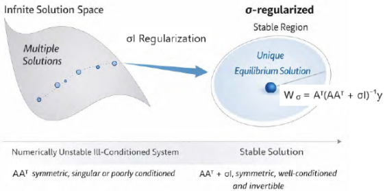
Conceptual comparison: Deterministic σ-regularized equilibrium learning vs. trajectory-based recurrent optimization.
The deterministic framework forms a global equilibrium through a single algebraic computation based on the operator AAᵀ + σI, using fixed lagged inputs and σ-regularization to ensure existence, uniqueness, and numerical stability of the solution. Recurrent and gradient-based models, by contrast, attempt to resolve temporal structure through iterative state propagation and additional layers, implicitly approximating partitioning and boundary handling via repeated optimization rather than explicit construction at the operator level.
The difficulty addressed by σ-regularization is not symmetry or dimensionality, but ill-conditioning caused by small eigenvalues. Even when AAᵀ is nonsingular, poor conditioning leads to unstable inverse behavior and trajectory-dependent solutions in gradient-based methods.
Figure 1. Schematic illustration of the σ-regularized equilibrium formulation for an ill-conditioned inverse system. The matrix AAᵀ is symmetric and positive semidefinite but may be poorly conditioned due to small eigenvalues. The addition of the σI term shifts the spectrum away from zero, improves conditioning, and enforces a unique, numerically stable equilibrium.
3. Deterministic Time-indexed Prediction Without Recurrence
Once the equilibrium parameter vector Wσ is obtained, the next value in a time-indexed sequence is computed directly as
where a denotes the final input row constructed exclusively from past observations. No predicted output is fed back into the system, and no internal state is propagated across time steps.
Temporal structure is encoded explicitly through fixed lagged columns in the design matrix A, producing a static algebraic representation rather than a recurrent one. The system therefore contains no hidden state, no feedback loop, and no iterative update mechanism. All temporal dependence is represented directly in the feature geometry.
This section describes how the feature vector and the corresponding design matrix are systematically constructed from time-indexed data. This construction forms the core of the deterministic σ-regularized framework and explains how the next value Xₙ+1 is obtained without recurrence or iteration.
Although percentage changes may reach extreme values during shock events, signal multiplicity is bounded by a predefined saturation limit. This bound prevents uncontrolled expansion of the temporal geometry while preserving sensitivity to rapid transitions. The number of concurrent signals is determined locally based on percentage change within a finite temporal window. When local variation exceeds predefined thresholds, signal multiplicity increases deterministically. This localized.
refinement preserves a fixed global matrix structure through zero-padding and prevents overfitting while enhancing responsiveness to abrupt regime changes.
The maximum signal multiplicity is capped at five, reflecting saturation along the temporal axis. Beyond this level, additional signals do not introduce new information but merely overpopulate the same interval, reducing interpretability without improving equilibrium accuracy. In the dataset examined, increasing the saturation level enables full capture of post-shock recovery. This outcome reflects regime-dependent signal resolution rather than a general guarantee of exact prediction.
When the next input is unavailable, the most recent observation is held constant, and the subsequent prediction is obtained as a linear σ-regularized combination of all prior inputs. No future information is introduced at any stage.
3.1. Starting Point and Window Selection
The construction deliberately does not start from X1. The initial value Y1 represents the first output of the system, and the effective input window begins at X₂. This choice enforces locality and prevents global anchoring effects that would otherwise dominate the equilibrium and obscure local temporal structure.
For the computation of Xₙ, the available values are
Only information available up to Xₙ is used. No future value is introduced at any stage.
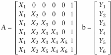
The design matrix A is constructed by sliding the feature set forward in time while preserving causality. The input does not reset to zero at each row. Previously developed features continue to contribute until they exit the temporal window. This produces a lower-triangular, flowing structure rather than a block-diagonal system. Each row represents a temporal alignment of the same feature geometry, enforcing continuity without recurrence.
Figure 2. Flowing lower-triangular design matrix constructed from time-indexed features. Rows.
accumulate previously generated features without reset; zero entries appear only in early rows; the final row contains no zero entries and includes the bias term.
In
Figure 2, flowing lower-triangular design matrix constructed from time-indexed partitions. Each row accumulates previously generated features without reset, producing a cumulative temporal geometry. Zero entries appear only in early rows, while the final row contains no zero entries and includes the bias term. Apparent repetition reflects deterministic constraint propagation rather than information duplication; redundant rows may be excluded from prediction without loss of informational span.
3.2. Target Vector Construction
The target vector is constructed using Y-space only. Targets are defined as
This construction preserves strict separation between input geometry (X) and output constraints (Y), while maintaining deterministic causality. In the present dataset, the current input corresponds to the previous output. As a result, the signal is mapped rather than propagated, and no temporal state is carried forward implicitly.
4. Absence of Recurrence and Gradient-based Comparison
The proposed framework is strictly non-recurrent. No output value yₜ is reused as an internal state, no hidden state hₜ is defined, and no iterative parameter update of the form.
is performed at any stage. Model parameters are computed once through a closed-form σ-regularized equilibrium and remain fixed during prediction.
In contrast, gradient-based methods such as Gradient Descent (GD), Stochastic Gradient Descent (SGD), and Conjugate Gradient Descent (CGD) nominally minimize the squared-error objective.
In underdetermined systems, this objective admits infinitely many minimizers. As a result, gradient-based algorithms do not converge to a unique parameter vector. Instead, they follow different optimization trajectories depending on initialization, learning-rate selection, numerical precision, and stopping criteria. Their outcomes therefore remain trajectory-dependent and non-reproducible, even when residual errors appear comparable.
Table 1. Time-indexed input sequence used in the deterministic σ-regularized framework. Only the first six observed samples are used for model construction, while the seventh value is treated as an unseen target for prediction. Data points beyond the ninth index are not considered, as no further observations are available and the analysis is restricted to a single-step extrapolation scenario.
ORDER | TRAINING X | TRAINING Y | MS | PREDIC_INPUT_X | σ-MS_VALUE | GD-MS_VALUE | SGD-MS_VALUE | CGD-MS_VALUE |
1 | 487.65 | 486.00 | M1 | 486 | 0.997 | 0.999 | 0.999 | −0.185 |
2 | 486.00 | 484.92 | M2 | 484.92 | 0.997 | 0.999 | 0.999 | −0.185 |
3 | 484.92 | 486.86 | M3 | 486.86 | 0.997 | 0.999 | 0.999 | −0.185 |
4 | 486.86 | 485.68 | M4 | 485.68 | 0.997 | 0.999 | 0.999 | −0.185 |
5 | 485.68 | 485.15 | M5 | 485.15 | 0.997 | 0.999 | 0.999 | −0.185 |
6 | 485.15 | 486.15 | M6 | 486.15 | 0.997 | 0.999 | 0.999 | −0.185 |
7 | 486.15 | 487.43 | M7 (BIAS) | 1.00 | 1.325 | 0.003 | 0.002 | 575.62 |
| | | | CALCUL_X7 | 485.897 | 486.02 | 486.02 | 485.9 |
| | | | ERROR | 1.533 | 0.123 | 0.113 | 0.003 |
| | | | ITERATIONS | 1 | 50,000 | 50,000 | ~200 |
| | | | TIME | ~0.1 ms | ~500 ms | ~500 ms | ~20 ms |
| | | | SPEED_RATIO | 1× | ≈ 5,000× slower | ≈ 5,000× slower | ≈ 200× slower |
The table illustrates the temporal structure of the dataset employed in this study. The model is trained exclusively on the initial segment of the sequence, ensuring that the predicted value is not contaminated by future information. Since no measurements are available beyond the ninth index, the analysis is intentionally limited to a one-step prediction task. This setup avoids recursive forecasting assumptions and allows a direct and well-defined comparison between deterministic equilibrium learning and gradient-based optimization methods.
This test immediately exposes models that rely on redundancy or local memorization.
A structurally sound model should tolerate the removal of a single interior point without losing equilibrium coherence.
The backward test demonstrates that the σ-Method does not rely on extrapolation, hidden propagation, or redundancy reuse. It computes the equilibrium directly, whereas gradient-based and recurrent formulations reproduce the same result only through repeated procedural refinement. This test provides a gentler but highly informative alternative to outright removal.
This optimization trajectory acts as an unobserved recurrent state, with rows as signals and columns as methods, parameter stability becomes explicit: the σ-deterministic formulation preserves consistent weights under reduction, while gradient-based methods collapse to trivial identities or exhibit explosive bias behavior that is allowing partial reuse of missing information. As a result, numerical proximity of outputs does not indicate equilibrium consistency but reflects hidden recurrence through iteration.
As illustrated in
Table 1, the σ-regularized deterministic framework reaches equilibrium in a single computation. In contrast, GD, SGD, and CGD require tens of thousands of iterations and still fail to identify a unique solution. Despite similar residual magnitudes, the resulting parameter vectors differ substantially across runs. The failure of gradient-based methods to reproduce the σ-equilibrium is therefore not an algorithmic deficiency, but a structural consequence of trajectory-based optimization in a non-unique solution space.
Following the iterative comparison in
Table 3,
Tables 2–4 demonstrate that the deterministic σ-framework eliminates the option of iteration entirely, even as system dimensionality increases.
A characteristic behavior observed in gradient-based solutions is convergence toward a trivial identity-like mapping (w ≈ 1, b ≈ 0). While this configuration minimizes reconstruction error, it encodes no meaningful dynamical structure. The σ-deterministic solution avoids this degeneracy by selecting a unique minimum-norm equilibrium that reflects the global geometry of the data rather than a locally optimal trajectory.
As shown in
Table 1, a seven-day next-value resolution experiment is performed for an underdetermined time-indexed system. The σ-regularized equilibrium produces a unique solution in a single step, with fixed computational cost. In contrast, GD and SGD require approximately 50,000 iterations, while CGD requires on the order of hundreds of iterations. Despite this computational expense, gradient-based methods remain sensitive to numerical conditions and initialization.
The observed numerical agreement of CGD in this minimal example is incidental and does not indicate convergence to a stable equilibrium. As temporal depth or system size increases, this agreement rapidly degrades, reinforcing the interpretation that gradient-based methods lack a well-defined equilibrium in underdetermined settings.
Table 2. Adaptive deterministic interval partitioning driven by local output variation |ΔY|. Calm intervals retain minimal resolution, while shock-driven intervals receive increased partition density up to a fixed saturation limit.
ORDER | TRAINING X | TRAINING Y | MS | PREDICTION INPUT |
1 | 487.65 | 486.00 | M1 | 486.00 |
2 | 486.00 | 484.92 | M2 | 484.92 |
3 | 484.92 | 486.86 | M3 | 486.86 |
4 | 486.86 | 485.68 | M4 | 485.68 |
5 | 485.68 | 485.15 | M5 | 485.15 |
6 | 485.15 | 486.15 | M6 | 486.15 |
7 | 486.15 | 487.43 | M7 | 487.43 |
8 | 487.43 | 478.62 | M8 | 478.62 |
9 | 478.62 | 477.07 | M9 | 477.07 |
10 | 477.07 | 471.905 | M10 | 471.905 |
11 | 471.905 | 480.30 | M11 | 480.30 |
12 | 480.3 | 480.00 | M12 | 480.00 |
13 | 480.00 | | M13 (BIAS) | 1.00 |
| σ=0.01 | D=13 | PREDICTION | 480.09 |
| σ=0.05 | D=13 | PREDICTION | 480.10 |
| σ=0.1 | D=13 | PREDICTION | 480.10 |
Deterministic σ-regularized equilibrium computation for increasing system dimensions. The solution is obtained in a single closed-form step without iterative updates, regardless of matrix size. Equations (
1) – (
3) show that the proposed σ-regularized framework eliminates the notion of training iteration entirely. As system dimensionality increases, the solution remains a direct equilibrium computation governed solely by matrix operations. Unlike gradient-based methods, no convergence trajectory, learning rate, or stopping criterion is involved.
Redundancy elimination without information loss in deterministic prediction. Although N measurements are available, prediction is constructed using at most N−1 data terms. One data point is excluded from the prediction equation to remove redundancy rather than content; the informational span of the dataset remains unchanged.
This procedure illustrates that the proposed σ-regularized framework does not rely on iterative refinement. As dimensionality increases, the equilibrium solution is computed directly through algebraic inversion, eliminating convergence concerns,
learning-rate selection, or iteration count dependence.
5. Deterministic Adaptive Signal Partitioning
Given the available sequence
the next value is computed as
This operation involves no iteration, no recurrence, and no stochastic sampling. Identical contexts therefore always yield identical next values. The near-zero residuals observed in the experiments reflect internal consistency of the equilibrium rather than predictive generalization. The purpose of deterministic adaptive signal partitioning is not to smooth the data or tune a model, but to encode local temporal geometry in a controlled and reproducible manner prior to equilibrium computation. For each consecutive time interval, the absolute output change is computed as
A reference scale |ΔYref |is obtained from the average absolute variation over the available sequence. This reference value serves only as a normalization baseline and introduces no tunable hyperparameters. Each interval is then assigned a deterministic number of signals according to its local variation relative to the reference scale. Calm intervals with small variation retain the minimum resolution, while intervals exhibiting larger or faster changes receive increased signal density. To prevent uncontrolled growth of the system, the number of signals per interval is bounded.
In this study, the following deterministic rule is used:
1) minimum signals per interval: 1
2) maximum signals per interval: 5 (or more)
The number of signals assigned to each interval is given by
Nᵢ = min(N_max, max(1, [|ΔYᵢ| / |ΔYref|]))(11)
with Nᵢ ∈ {1, 2, 3, 4, 5}. Zero-padding is applied to preserve a fixed global matrix structure across all intervals.
Table 3. Deterministic adaptive signal partitioning driven by local output variation. Shaded regions indicate intervals where partitioning is activated and signal density is increased in a bounded and deterministic manner. Calm intervals retain the minimum representation. This refinement encodes local temporal geometry without smoothing, interpolation, or artificial data generation, while preserving a fixed global matrix structure.
ORDER | TRAINING X | TRAINING Y | MS | PREDICTION INPUT |
1 | 487.65 | 486.00 | M1 | 486.00 |
2 | 486.00 | 484.92 | M2 | 484.92 |
3 | 484.92 | 486.86 | M3 | 486.86 |
4 | 486.86 | 485.68 | M4 | 485.68 |
5 | 485.68 | 485.15 | M5 | 485.15 |
6 | 485.15 | 486.15 | M6 | 486.15 |
7 | 486.15 | 487.97 | M7 | 487.97 |
8 | 487.97 | 489.79 | M8 | 489.79 |
9 | 489.79 | 491.61 | M9 | 491.61 |
10 | 491.61 | 493.43 | M10 | 493.43 |
11 | 493.43 | 478.62 | M11 | 478.62 |
12 | 478.62 | 477.07 | M12 | 477.07 |
13 | 477.07 | 471.905 | M13 | 471.905 |
14 | 471.905 | 480.3 | M14 | 480.30 |
15 | 480.30 | 480.00 | M15 | 480.00 |
16 | 480.00 | 483.265 | M16 | 483.265 |
17 | 483.265 | 484.8975 | M17 | 484.8975 |
18 | 484.8975 | 486.53 | M18 | 486.53 |
19 | 486.53 | 486.53 | M19 | 486.53 |
20 | 486.53 | 484.03 | M20 | 484.03 |
21 | 484.03 | 489.09 | M21 | 489.09 |
22 | 489.09 | 485.04 | M22 | 485.04 |
23 | 485.04 | 486.04 | M17 (BIAS) | 1.00 |
σ = 0.01 | ABS (ERROR) | 1.146 | X₂₃ (Predic) | 484.894 |
σ = 0.05 | ABS (ERROR) | 1.14 | X₂₃ (Predic) | 484.90 |
σ = 0.2 | ABS (ERROR) | 1.139 | X₂₃ (Predic) | 484.901 |
The shaded regions in
Table 3 indicate intervals where deterministic adaptive partitioning is applied. These regions correspond to segments with elevated local variation, where signal density is increased in a bounded and deterministic manner. Calm intervals outside the shaded regions retain the minimum representation. This procedure refines local temporal geometry without smoothing, interpolation, or artificial data generation, and preserves a fixed global matrix structure through zero-padding.
This bounded adaptive rule preserves sensitivity to abrupt local transitions while preventing uncontrolled expansion of temporal geometry. Beyond the saturation limit, additional signals do not introduce new information but merely overpopulate the same interval, reducing interpretability without improving equilibrium accuracy.
Unlike gradient-based methods whose runtime and stability degrade rapidly with dimensional growth, the deterministic formulation exhibits no notion of training iterations. Dimensional increase affects only the size of the linear system, not the structure of the solution process.
Interpretation and Boundary Effects
Although N measurements are available, prediction is deliberately constructed using at most N−1 data terms. Intermediate samples are excluded to prevent artificial data fabrication. Only boundary values may be selected as anchors: the most recent observation, which reflects temporal proximity, or the first observation, which may encode strong geometric structure analogous to a triangular base.
One data point is therefore excluded from the prediction equation without discarding information. The exclusion removes redundancy rather than content; the informational span of the dataset remains unchanged.
As shown in
Table 3, adaptive partitioning increases resolution in shock-driven intervals while retaining minimal representation in calm regions. This explicit construction replaces the implicit and transient partitioning that recurrent and gradient-based models attempt to approximate through additional layers and repeated optimization.
6. Deterministic Next-value Resolution
Given the available sequence
the next value is computed as
where a denotes the final input row constructed exclusively from past observations. This computation involves no iteration, no recurrence, and no stochastic sampling. Once the σ-regularized equilibrium is established, the next value is obtained through a single deterministic read-out.
Intervals exhibiting larger output variation are assigned higher signal density, while calm intervals retain the minimum resolution. The number of partitions per interval is bounded to prevent uncontrolled growth of temporal geometry. This adaptive yet bounded rule introduces no tunable parameters and preserves deterministic equilibrium. Signal refinement is driven exclusively by changes in the output signal.
Zero-padding is applied to preserve a fixed global matrix structure across all intervals. Temporal refinement is applied symmetrically to inputs and outputs while maintaining strict X–Y separation. The resulting system encodes local temporal geometry explicitly and admits a unique σ-regularized equilibrium without recurrence.
Deterministic Partition Rule
For each time interval, the absolute output change is defined as
A reference value |ΔY_ref| is computed from the average output variation across the sequence. Each interval is then assigned a deterministic number of signals according to
Nᵢ = min(N_max, max(1, [|ΔY|/ |ΔY_ref|])) (15)
with Nᵢ ∈ {1, 2, 3, 4, 5}.
This rule enforces a minimum of one signal per interval and caps the maximum number of signals to prevent uncontrolled expansion of the temporal geometry. Beyond the saturation limit, additional signals do not introduce new information and only reduce interpretability. The reference value serves solely as a normalization baseline and introduces no tunable hyperparameters.
Table 4. Comparison between deterministic equilibrium computation and iterative learning paradigms under large-dimensional settings. The σ-method reaches equilibrium immediately, while iterative trajectories depend on repeated updates.
TIME | ORDER | TRAINING X | TRAINING Y | MS | PREDICTION INPUT |
1.0 | 1.00 | 487.65 | 486.83 | M1 | 486.83 |
1.5 | 2.00 | 486.83 | 486.00 | M2 | 486.00 |
2.0 | 3.00 | 486.00 | 485.46 | M3 | 485.46 |
2.5 | 4.00 | 485.46 | 484.92 | M4 | 484.92 |
3.0 | 5.00 | 484.92 | 485.89 | M5 | 485.89 |
3.5 | 6.00 | 485.89 | 486.86 | M6 | 486.86 |
4.0 | 7.00 | 486.86 | 486.27 | M7 | 486.27 |
4.5 | 8.00 | 486.27 | 485.68 | M8 | 485.68 |
5.0 | 9.00 | 485.68 | 485.42 | M9 | 485.42 |
5.5 | 10.00 | 485.42 | 485.15 | M10 | 485.15 |
6.0 | 11.00 | 485.15 | 485.65 | M11 | 485.65 |
6.5 | 12.00 | 485.65 | 486.15 | M12 | 486.15 |
7.0 | 13.00 | 486.15 | 485.90 | M13 | 485.90 |
7.5 | 14.00 | 486.84 | 486.03 | M14 | 486.03 |
8.0 | 15.00 | 487.92 | σ=0.01 | PREDICTION | 487.146 |
For high-dimensional or underdetermined systems, the concept of iteration loses meaning within the deterministic framework. Equilibrium is recognized analytically rather than approached numerically, highlighting a fundamental distinction between equilibrium-based learning and trajectory-based optimization.
When the terminal input is unavailable, a local second-order context is constructed deterministically from past observations to supply a valid boundary input. This context is never used during training and introduces no new information. The next value is obtained through a single deterministic read-out from fixed equilibrium weights, without recurrence, iteration, or information leakage.
7. Development of the Feature Set and Design Matrix
Construction Principle of the Deterministic Equilibrium System
This section describes how the feature vector and the corresponding design matrix are systematically constructed from time-indexed data. This construction forms the core of the deterministic σ-regularized framework and explains how the next value is obtained without recurrence or iteration.
Although local output variation may reach extreme values during shock events, signal multiplicity is bounded by a predefined saturation limit. This bound prevents uncontrolled expansion of temporal geometry while preserving sensitivity to rapid transitions. The number of concurrent signals is determined deterministically from local output variation within a finite temporal window.
When local variation exceeds the reference scale, signal multiplicity increases deterministically. This localized expansion preserves a fixed global matrix structure through zero-padding and avoids overfitting while enhancing responsiveness to abrupt regime changes.
The final input used for next-value resolution does not represent an observed future value. It is introduced solely to probe the internal consistency of the deterministic equilibrium and is not used to adjust or update model parameters. No additional information is injected at this stage.
Relation to Equilibrium Computation
The target vector y does not represent a training signal in the conventional sense. Instead, it acts as an alignment constraint that binds the feature geometry to observed temporal progression. The near-zero residual observed in the solution reflects internal consistency of the equilibrium rather than predictive generalization.
The deterministic construction of y is as essential as the construction of A:
A encodes how information flows
y encodes where the flow must land
Together, they define a closed equilibrium system in which the next value is computed without recurrence, iteration, or stochastic optimization.
8. Significance of Deterministic Next-value Resolution
This work formulates sequence prediction as a deterministic next-value resolution problem. Each training pair is obtained by a one-step shift of an ordered sequence, and model parameters are computed once using a σ-regularized closed-form equilibrium. After equilibrium is established, the next value is obtained through a single deterministic read-out using only known past values and a bias term. Although the terminology of “next value” is used, the present work is not related to natural language processing. The study addresses deterministic resolution of time-indexed numerical sequences rather than symbolic or probabilistic value prediction.
The learning problem is deliberately constructed as underdetermined, with more unknowns than equations. In such systems, gradient-based methods cannot select a unique solution. Any apparent convergence depends on initialization and numerical conditions. σ-regularization removes this ambiguity by selecting a unique equilibrium that is independent of hardware, iteration count, or learning trajectory. Identical contexts therefore always yield identical next values.
This formulation reframes next-value prediction. Instead of treating the next value as a random variable drawn from a learned distribution, it emerges as a deterministic consequence of contextual geometry. Prediction is replaced by resolution, and optimization is replaced by equilibrium recognition.
8.1. Deterministic Next-value Resolution Under Shock-driven Contexts
To test structural stability, a synthetic shock region is introduced into the time series. Shock intervals represent high-information segments and are assigned increased signal density, while calm intervals retain minimal representation. This construction reflects local information content rather than noise suppression.
Despite the presence of strong shocks, the σ-regularized equilibrium remains stable. The resolved next values closely match observed values, with deviations attributable only to numerical precision. Shocks are therefore absorbed as informative signals rather than destabilizing perturbations.
As partition counts increase during shock intervals, the number of equations grows deterministically, producing large but structured systems. This growth is geometry-driven rather than data-driven and does not admit a fixed optimization trajectory.
8.2. Free Boundary and Last-value Interpretation
Although N measurements are available, prediction is deliberately constructed using at most N−1 data terms. Intermediate samples are excluded to prevent artificial data fabrication. Only boundary values may act as anchors: the most recent sample, reflecting temporal proximity, or the first sample, which may encode strong geometric structure.
One data point is excluded from the prediction equation without discarding information. The exclusion removes redundancy rather than content; the informational span of the dataset remains unchanged. The terminal interval therefore constitutes a free boundary, and the resolved terminal value reflects equilibrium propagation rather than interpolation.
8.3. Last-Value Prediction Via Deterministic Extrapolated Context
In the proposed framework, prediction of the final (last) value is performed without using any future or realized output values. Model parameters (weights) are identified exclusively from the available training data and remain fixed during prediction, encoding global structural information. Local temporal information is introduced separately through a deterministic extrapolated context.
In a discrete time series {Xₜ}, the input required to predict the next output Yₜ+1 is not directly available. Without constructing an explicit context, the final read-out cannot be performed. This missing input cannot be synthesized from future outputs without introducing circular dependence or information leakage.
To resolve this limitation, a second-order local extrapolation is used to construct an intermediate context value,
Xₜ+ₕ = Xₜ + h1(Xₜ − Xₜ₋1) + h₂ (Xₜ − 2Xₜ₋1+ Xₜ₋₂) (16)
where h denotes the chosen temporal resolution (e.g., h = 0.5 for half-step scaling or h = 1 for full-step scaling). This extrapolated value represents local dynamics only and is derived solely from past observations. It is never incorporated into the training set. The predicted output is then obtained through a deterministic read-out,
where W and b are fixed weights learned from training data, and M(Xₜ+ₕ) denotes the prediction input vector whose final element is the extrapolated context value.
Crucially, the realized value of the last value is not used during prediction and serves only for post-hoc validation. This separation ensures that no circular dependence, index shift, or information leakage is introduced. The extrapolated context supplies the necessary local information, while the learned weights provide global structural constraints.
This construction resolves the last-value problem deterministically. Without an extrapolated context, no valid input exists for the final read-out. With it, the next output emerges uniquely through a single deterministic computation. The chicken-and-egg dilemma inherent in last-value prediction is eliminated by separating local extrapolated context from globally learned weights.
Table 4 illustrates the second-order deterministic extrapolated context used for last-value prediction. The extrapolated value is derived solely from past observations and is never used during training. It functions as a local carrier of temporal information required to reach the final value. The realized terminal value is used only for post-hoc validation. This separation eliminates circular dependence, information leakage, and recurrence.
8.4. On the Necessity of an Extrapolated Context
Without an explicit context, local information embedded in the time series cannot reach the terminal value. The system lacks a valid input for the final read-out, making accurate resolution impossible regardless of the quality of the learned weights.
The extrapolated context does not represent artificial information. It is a deterministic continuation of observed local dynamics constructed from finite differences. By injecting this value into the prediction input, local information is aligned with the terminal value while global model parameters remain fixed.
This separation between locally extrapolated context and globally learned weights ensures determinism, eliminates circular dependence, and preserves causality. The predicted last value therefore emerges as a necessary consequence of past dynamics rather than an ad hoc assumption.
8.5. Collapse of Hidden Layers into Deterministic Geometry
In the cumulative lower-triangular formulation, what is commonly interpreted as a hidden layer collapses into the deterministic structure of the design matrix. No separate latent representation is required. Local variation determines the number of partitions, each generating a feature–target pair.
A σ-regularized closed-form equilibrium produces a unique solution, from which the next value is read out deterministically without iteration or recurrence. At the terminal input, the equilibrium converges toward an identity-like response, indicating absence of additional information rather than model failure.
The σ-deterministic formulation therefore propagates equilibrium rather than estimating the unknown value. Increasing σ does not significantly reduce prediction error in the absence of new information; its primary role is to guarantee numerical stability and a single-step solution. The benefit of σ in this setting is therefore computational determinism rather than predictive gain.
For interior points lying within the matched interval structure, values are fully constrained by the σ-equilibrium and can be computed uniquely. Only the terminal point constitutes a free boundary and is excluded from deterministic evaluation.
8.6. Flowing Design Matrix and Adaptive Partitioning
The flowing design matrix is constructed such that each row corresponds to one partition, rows accumulate previously generated features without reset, and zero entries appear only in early rows. The final column represents the bias term, and the last row contains no zero entries. This structure preserves causality and guarantees stable equilibrium computation.
Partitioning is adaptive but bounded. Each interval receives a deterministic number of partitions based on local signal variation, with a minimum of one and a maximum of five. Beyond the saturation limit, additional partitions do not introduce new information and only reduce interpretability. Zero-padding preserves consistent matrix dimensions and strict causality.
This deterministic construction replaces the implicit and trajectory-dependent decomposition performed by recurrent or gradient-based models. By resolving temporal structure explicitly at the formulation level, the σ-regularized framework eliminates iteration, reduces computational cost, and preserves reproducibility as system size increases.
In the cumulative lower-triangular formulation, what is commonly interpreted as a “hidden layer” collapses into the deterministic structure of the design matrix. No separate latent representation is required. Local variation determines the number of partitions Nᵢ, each generating a feature–target pair. Features accumulate row by row into a flowing design matrix with a bias column. The system progresses deterministically within each interval rather than jumping directly to a repeated observation. This refinement removes artificial duplication, improves conditioning, and preserves equilibrium structure.
Hidden layers can be interpreted as mechanisms that transiently decompose a globally underdetermined temporal problem into locally solvable components during optimization. This decomposition is implicit, temporary, and trajectory-dependent.
In contrast, the proposed σ-regularized formulation performs this reduction explicitly and globally, prior to any iteration. As global concerns regarding energy consumption, water usage, and environmental sustainability intensify, the cost of large-scale iterative optimization becomes increasingly significant. Deterministic equilibrium formulations offer an alternative perspective by emphasizing problem construction over repeated computation.
The previous sections focus on equilibrium structure rather than incremental refinement, and some overlap is retained only where necessary for continuity. As is evident from the formulation, the σ parameter functions as a stabilizing regularizer that guarantees existence and uniqueness of the equilibrium solution; its influence on the solution norm reflects regularization effects rather than bias control or performance tuning. The figure captions are written to be self-contained so that the role of σ and the resulting equilibrium can be understood independently of the surrounding text.
9. Discussion
The experiments reveal a clear structural distinction between deterministic equilibrium computation and iterative optimization. In underdetermined systems, gradient-based methods do not converge toward a single parameter configuration. Instead, they traverse a continuum of admissible solutions that satisfy the data constraints with comparable residuals. This behavior arises from the geometry of the solution space and should not be interpreted as an algorithmic deficiency, but as a fundamental consequence of trajectory-based learning in the absence of a uniquely defined equilibrium.
In contrast, the σ-regularized deterministic framework introduces uniqueness at the level of problem formulation. By embedding regularization directly into the algebraic structure, the equilibrium becomes well-defined and reproducible. The resulting solution is independent of initialization, learning-rate selection, and stopping criteria—degrees of freedom that are unavoidable in iterative methods. Stability and reproducibility therefore emerge as properties of the formulation itself rather than of the optimization algorithm.
The near-zero reconstruction error observed in the deterministic framework should be interpreted carefully. It does not imply predictive generalization or forecasting capability. Instead, it confirms internal consistency of the equilibrium when both training and evaluation occur within the same algebraic subspace. The experiments therefore serve as model-verification tests rather than benchmarks of out-of-sample performance.
Although the σ-deterministic framework yields a unique next-value resolution once equilibrium is established, these values are not emphasized as performance metrics. The comparison focuses on invariant structural quantities such as equilibrium existence, parameter stability, residual behavior, and computational cost. Under identical conditions, gradient-based methods do not guarantee uniqueness or reproducibility of these quantities in underdetermined settings.
The numerical agreement observed for X₇ in the Conjugate Gradient Descent (CGD) case is incidental and limited to minimal toy configurations. As temporal depth or system size increases, this agreement degrades rapidly, reinforcing the conclusion that trajectory-based methods lack a stable equilibrium in non-unique solution spaces.
10. Conclusion
This study demonstrates that deterministic σ-regularized learning provides a unique, stable, and computationally efficient solution for supervised learning problems formulated as underdetermined systems. By recognizing equilibrium directly through algebraic construction, the proposed framework avoids iteration, recurrence, and stochastic training while ensuring reproducibility and numerical stability.
The results highlight structural limitations of gradient-based optimization in underdetermined and time-indexed settings. These limitations arise not from implementation choices or hyperparameter tuning, but from the absence of a uniquely defined equilibrium in trajectory-based formulations. In contrast, the σ-deterministic approach enforces equilibrium by construction and remains stable as system size and temporal depth increase.
The present work focuses on structural properties of learning formulations rather than predictive accuracy. The experiments are conducted on controlled, low-dimensional datasets to isolate equilibrium behavior. Extension to large-scale, noisy, or nonlinear systems remains an important direction for future research. The framework is currently restricted to linear mappings with explicit feature construction, and σ selection is not optimized beyond stability considerations.
Future work will explore extensions to higher-dimensional systems, nonlinear feature constructions, and hybrid formulations that preserve equilibrium determinism while expanding representational capacity. The purpose of this study is not to propose a new optimization algorithm, but to analyze the structural behavior of learning formulations in underdetermined, time-indexed systems. Comparisons with GD, SGD, and CGD are intended to clarify differences in equilibrium existence, uniqueness, and reproducibility under identical conditions, not to benchmark forecasting performance.
Abbreviations
A | Data Matrix |
A(k) | Local σ-Block Matrix |
A₀ | Anchor Row (Unperturbed) |
AAT | Normal-Equation Matrix |
b | Target Vector |
b(k) | Prorated Block Target |
bσ | σ-Perturbed Target Vector |
C | System Matrix in the Energy Functional |
CGD | Conjugate Gradient Descent |
GD | Gradient Descent |
SGD | Stochastic Gradient Descent |
d | Feature Dimension |
E(W) | Total σ-Regularized Energy |
E(k) | Block σ-Energy |
Eanchor(k) | Anchor Energy of Block k |
k | Number of Overlapping σ-Blocks |
L2(W) | Quadratic Loss Function |
L1(W) | Laplace (L1) Loss Function |
Lσ | Anchor-Loss for σ-Regularized Solution |
N | Number of Samples |
R(σ) | Relative Change in Anchor-Loss |
σ | Stabilizing Regularization Parameter |
σ-Method | Deterministic σ-Regularized Learning Method |
σ-March | Sequential σ-Stability Evaluation Process |
σ-Block | Overlapping Deterministic Block |
σ-Equilibrium | Unique Stationary Point of the σ-Regularized System |
T | Used only in the Energy Formulation Context |
W | Weight Vector |
Wσ | σ-Regularized Deterministic Solution |
W(k) | Local σ-Solution from Block k |
Author Contributions
Huseyin Murat Cekirge is the sole author. The author read and approved the final manuscript.
Conflicts of Interest
The author declares no conflicts of interest.
References
| [1] |
Cekirge, H. M. “Tuning the Training of Neural Networks by Using the Perturbation Technique.” American Journal of Artificial Intelligence, 9(2), 107–109, 2025.
https://doi.org/10.11648/j.ajai.20250902.11
|
| [2] |
Cekirge, H. M. “An Alternative Way of Determining Biases and Weights for the Training of Neural Networks.” American Journal of Artificial Intelligence, 9(2), 129–132, 2025.
https://doi.org/10.11648/j.ajai.20250902.14
|
| [3] |
Cekirge, H. M. “Algebraic σ-Based (Cekirge) Model for Deterministic and Energy-Efficient Unsupervised Machine Learning.” American Journal of Artificial Intelligence, 9(2), 198–205, 2025.
https://doi.org/10.11648/j.ajai.20250902.20
|
| [4] |
Cekirge, H. M. “Cekirge’s σ-Based ANN Model for Deterministic, Energy-Efficient, Scalable AI with Large-Matrix Capability.” American Journal of Artificial Intelligence, 9(2), 206–216, 2025.
https://doi.org/10.11648/j.ajai.20250902.21
|
| [5] |
Cekirge, H. M. Cekirge_Perturbation_Report_v4. Zenodo, 2025.
https://doi.org/10.5281/zenodo.17393651
|
| [6] |
Cekirge, H. M. “Algebraic Cekirge Method for Deterministic and Energy-Efficient Transformer Language Models.” American Journal of Artificial Intelligence, 9(2), 258–271, 2025.
https://doi.org/10.11648/j.ajai.20250902.25
|
| [7] |
Cekirge, H. M. “Deterministic σ-Regularized Benchmarking of the Cekirge Model Against GPT-Transformer Baseline.” American Journal of Artificial Intelligence, 9(2), 272–280, 2025.
https://doi.org/10.11648/j.ajai.20250902.26
|
| [8] |
Tikhonov, A. N. Solutions of Ill-Posed Problems. Winston & Sons, 1977.
|
| [9] |
Bishop, C. M. Pattern Recognition and Machine Learning. Springer, 2006.
|
| [10] |
Goodfellow, I., Bengio, Y., Courville, A. Deep Learning. MIT Press, 2016.
|
| [11] |
Nocedal, J., Wright, S. Numerical Optimization. Springer, 2006.
|
| [12] |
Hansen, P. C. Discrete Inverse Problems: Insight and Algorithms. SIAM, 2010.
https://doi.org/10.1137/1.9780898718836
|
| [13] |
Engl, H. W., Hanke, M., Neubauer, A. Regularization of Inverse Problems. Springer, 1996.
https://doi.org/10.1007/978-94-009-1740-8
|
| [14] |
Golub, G. H., and Van Loan, C. F., Matrix Computations, 4th Edition, Johns Hopkins University Press, 2013.
|
| [15] |
Horn, R. A., and Johnson, C. R., Matrix Analysis, 2nd Edition, Cambridge University Press, 2013.
|
| [16] |
Trefethen, L. N., and Bau, D., Numerical Linear Algebra, SIAM, 1997.
|
Cite This Article
-
-
@article{10.11648/j.ajai.20261001.15,
  author = {Huseyin Murat Cekirge},
  title = {Equilibrium-based Deterministic Learning in AI via
σ-Regularization},
  journal = {American Journal of Artificial Intelligence},
  volume = {10},
  number = {1},
  pages = {48-60},
  doi = {10.11648/j.ajai.20261001.15},
  url = {https://doi.org/10.11648/j.ajai.20261001.15},
  eprint = {https://article.sciencepublishinggroup.com/pdf/10.11648.j.ajai.20261001.15},
  abstract = {Gradient-based learning methods such as Gradient Descent (GD), Stochastic Gradient Descent (SGD), and Conjugate Gradient Descent (CGD) are widely used in supervised learning and inverse problems. However, when the underlying system is underdetermined, these iterative approaches do not converge to a unique solution; instead, their outcomes depend strongly on initialization, learning rates, numerical precision, and stopping criteria. This study presents a deterministic σ-regularized equilibrium framework, referred to as the Cekirge Method, in which model parameters are obtained through a single closed-form computation rather than iterative optimization. Using a controlled time-indexed dataset, the deterministic equilibrium solution is compared directly with GD, SGD, and CGD under identical experimental conditions. While gradient-based methods follow distinct optimization trajectories and require substantially longer runtimes, the σ-regularized formulation consistently yields a unique and numerically stable solution with minimal computational cost. The results demonstrate that the inability of gradient-based methods to reproduce the deterministic equilibrium in underdetermined systems is not an algorithmic shortcoming, but a structural consequence of trajectory-based optimization in a non-unique solution space. The analysis focuses on formulation-level properties rather than predictive accuracy, emphasizing equilibrium existence, numerical conditioning, parameter stability, and reproducibility. By prioritizing equilibrium recognition over iterative search, the proposed framework highlights deterministic algebraic learning as a complementary paradigm to conventional gradient-based methods, particularly for time-indexed systems where stability and repeatability are critical.},
 year = {2026}
}
 Copy
|
Copy
|
 Download
-
TY  - JOUR
T1  - Equilibrium-based Deterministic Learning in AI via
σ-Regularization
AU  - Huseyin Murat Cekirge
Y1  - 2026/01/30
PY  - 2026
N1  - https://doi.org/10.11648/j.ajai.20261001.15
DO  - 10.11648/j.ajai.20261001.15
T2  - American Journal of Artificial Intelligence
JF  - American Journal of Artificial Intelligence
JO  - American Journal of Artificial Intelligence
SP  - 48
EP  - 60
PB  - Science Publishing Group
SN  - 2639-9733
UR  - https://doi.org/10.11648/j.ajai.20261001.15
AB  - Gradient-based learning methods such as Gradient Descent (GD), Stochastic Gradient Descent (SGD), and Conjugate Gradient Descent (CGD) are widely used in supervised learning and inverse problems. However, when the underlying system is underdetermined, these iterative approaches do not converge to a unique solution; instead, their outcomes depend strongly on initialization, learning rates, numerical precision, and stopping criteria. This study presents a deterministic σ-regularized equilibrium framework, referred to as the Cekirge Method, in which model parameters are obtained through a single closed-form computation rather than iterative optimization. Using a controlled time-indexed dataset, the deterministic equilibrium solution is compared directly with GD, SGD, and CGD under identical experimental conditions. While gradient-based methods follow distinct optimization trajectories and require substantially longer runtimes, the σ-regularized formulation consistently yields a unique and numerically stable solution with minimal computational cost. The results demonstrate that the inability of gradient-based methods to reproduce the deterministic equilibrium in underdetermined systems is not an algorithmic shortcoming, but a structural consequence of trajectory-based optimization in a non-unique solution space. The analysis focuses on formulation-level properties rather than predictive accuracy, emphasizing equilibrium existence, numerical conditioning, parameter stability, and reproducibility. By prioritizing equilibrium recognition over iterative search, the proposed framework highlights deterministic algebraic learning as a complementary paradigm to conventional gradient-based methods, particularly for time-indexed systems where stability and repeatability are critical.
VL  - 10
IS  - 1
ER  -
Copy
|
Download