Modelling Dekadal Rainfall Dynamics in Kenyan Subnational Regions Using Sarima Model

Linnet Chege; Peter Gachoki; Joseph Eyang’an Esekon

doi:doi:10.11648/j.ajtas.20261504.14

Research Article |

| Peer-Reviewed

Modelling Dekadal Rainfall Dynamics in Kenyan Subnational Regions Using Sarima Model

Linnet Chege^*

, Peter Gachoki, Joseph Eyang’an Esekon

Published in American Journal of Theoretical and Applied Statistics (Volume 15, Issue 4)

Received: 30 June 2026 Accepted: 14 July 2026 Published: 6 August 2026

Views: Downloads:

Download PDF

Share This Article

Twitter
Linked In
Facebook

Abstract

Kenya is very weather sensitive, and the seasonality and variability of rainfall has a significant impact on agricultural productivity, water resource management and food security. Therefore, precise rainfall prediction is a key requirement for climate risk management and decision-making. Most Kenyan rainfall studies have been of monthly and/or annual rainfall, which may not be sensitive enough to the intra-seasonal variability in rainfall seen at dekadal (10-day) time scales. The aim of this study was to model and forecast dekadal rainfall dynamics in selected Sub-national regions of Kenya using Seasonal Autoregressive Integrated Moving Average (SARIMA) models. The quantitative time series research design adopted involved Box–Jenkins methodology with data on dekadal rainfall from 2021 to 2025 from the Humanitarian Data Exchange (HDX). The five regions namely Manyatta, Mbeere North, Igembe Central, Marsabit and Isiolo were chosen for analysis. Data was analyzed by R statistical software. Logarithmic transformation and differencing were used to stabilize the variance and to make the data stationary as verified by the Augmented Dickey–Fuller test. Autocorrelation Function (ACF) and Partial Autocorrelation Function (PACF) were used to identify the candidate SARIMA models, while Akaike Information Criterion (AIC) and Bayesian Information Criterion (BIC) were used to select the models. Model adequacy was checked with residual diagnostics and Ljung–Box test, and the forecasting performance was judged based on RMSE, MAE, MAPE, and MASE. The results showed that SARIMA (1,0,0) (1,1,1)₃₆was the most suitable model for regions51348,51352, and51364, whereas SARIMA (1,0,0) (0,1,1)₃₆ provided the best fit for regions 51357 and 51363. Residual diagnostics also showed that the models estimated were appropriate to represent the temporal dependence in the rainfall series, as the residuals were in the form of white noise. High MAPE values were observed, which were mostly related to the intermittent nature of the rainfall data, but satisfactory forecasting performance was shown by RMSE, MAE and MASE. Forecasts for the coming year reproduced the observed seasonal rainfall pattern and showed greater uncertainty in the longer-term forecasts. In general, the chosen SARIMA models were successful in modelling dekadal rainfall patterns and can be a valuable tool for agricultural planning, water resource management, and climate risk preparedness for Kenya.

Published in	American Journal of Theoretical and Applied Statistics (Volume 15, Issue 4)
DOI	10.11648/j.ajtas.20261504.14
Page(s)	149-163
Creative Commons	This is an Open Access article, distributed under the terms of the Creative Commons Attribution 4.0 International License (http://creativecommons.org/licenses/by/4.0/), which permits unrestricted use, distribution and reproduction in any medium or format, provided the original work is properly cited.
Copyright	Copyright © The Author(s), 2026. Published by Science Publishing Group

Keywords

Rainfall Variability, Dekadal Rainfall, SARIMA Modelling, Rainfall Forecasting

1. Introduction

Rainfall variability in Eastern Africa is influenced by complex interactions between oceanic and atmospheric drivers, which shape both interannual and intra-seasonal variability. Relation between Indian Ocean Dipole and ENSO moderate rainfall anomalies in Eastern Africa and influence when seasonal rainfall occur and its intensity

[1]

. Regional contrasts in rainfall over Africa, based on long-term satellite measurements, emphasize the role of localized rainfall modelling methods that are able to capture sub-seasonal variability that can be of value in agricultural and water management decision-making

[2]

An intermediate temporal scale such as dekadal rainfall provides a convenient balance between time and data continuity. Dekadal aggregation preserves the information on the onset, offset and persistence of dry spells in daily rainfall series, while reducing random noise present in daily rainfall series. The study by

[3]

revealed that the variability of seasonal rainfall in East Africa is strongly correlated to the global sea surface temperature deviations, indicating that the sub-seasonal rainfall processes are responsive to large-scale climate drivers.

[4]

, further identified dekadal rainfall variability over East Africa associated with oceanic forcing mechanisms. These results suggest that the variability of rainfall exists at several time scales, and therefore, dekadal data can be used to extract significant climate variants that can be used to forecast the seasons.

The study by

[5]

, evaluated the applicability of SARIMA models to examine and predict the trend in monthly rainfall in Embu County, Kenya using data on monthly rainfall that was available in 1998-2017. Prior time-series analysis indicated a high level of non-stationarity and high seasonality at the yearly level, which indicate the presence of a bimodal rainfall regime in the region. In order to address these characteristics, the authors used both non-seasonal and seasonal differencing, ACF and PACF plots to guide model identification. A number of SARIMA models were fitted and analyzed using Akaike Information Criterion (AIC) and residual diagnostic inspection. SARIMA (1,1,1) (0,1,2)₁₂ was the best model identified in the study since the residuals in the model showed white-noise behavior and the model gave precise forecasts for short-term rainfall. The results showed that SARIMA models can account for seasonal variations in rainfall, and provide an effective forecasting instrument in agricultural planning, drought preparedness and water-resource management in Embu County and similar regions.

Although a number of studies have been done using SARIMA models to forecast rainfall in Kenya and neighboring East African nations, there are still gaps. Dekadal rainfall series have been underreported, as most studies have investigated monthly or annual data, which limits understanding of intra-seasonal variability critical for agriculture and water resource management. Existing studies are often localized, covering only single counties or stations, which does not necessarily allow the research to capture spatial variability in seasonal rainfall patterns. There is limited research on whether a single SARIMA system can be effective in different climatic areas in Kenya. The objectives of this study were to fit a SARIMA model to dekadal rainfall data, to assess model performance using diagnostic measures and to generate rainfall forecasts with quantified uncertainty.

2. Methodology

Rainfall data, covering the period January 2021 to December 2025, that was used in this study was accessed through Humanitarian Data Exchange (HDX) which provided the dekadal (10-day) rainfall estimates on the subnational level in Kenya. The dekadal time resolution yielded 36 observations in a year and therefore was appropriate in SARIMA modelling.

2.1 Data Pre-processing

2.1.1. Exploratory Data Analysis

Summary statistics per region were computed and the selection of regions was done based on statistical parameters such as the coefficient of variation, standard deviation and the mean rainfall.

2.1.2. Time Series Visualization

The plotting of the rainfall series provided the ability to determine the seasonal peaks, dry seasons, and extreme rainfall seasons which are major features that are focused on in SARIMA models. Visual inspection was used in spotting outliers, missing values and structural breaks that could impact on the model performance and forecast accuracy.

2.1.3. Variance Transformation

Let the dekadal rainfall time series be defined as:

\{R t\}, t = 1, 2 \dots, n

(1)

Where;

R t

= rainfall (mm) recorded in the t-th dekad (10-day period)

n

= total number of dekads observed

To stabilize variance, a logarithmic transformation was applied:

X t = \log (R t + 1)

(2)

where

X t

is the transformed rainfall series.

2.1.4. Stationarity and Differencing

The rainfall series was tested for stationarity using the Augmented Dickey-Fuller (ADF) test.

Δ X_{t} = α + βt + γ X_{t - 1} + \sum_{i = 1}^{k} δ_{i} Δ X_{t - i} + ε_{t}

(3)

The hypotheses for the test were:

H_{0} : γ = 0

(4)

H_{1} : γ < 0

(5)

Where the null hypothesis

H_{0} : γ = 0

means the series has a unit root, indicating non stationarity whereas

H_{1} : γ < 0

means the series does not have a unit root hence stationary. If non-stationarity was detected, the rainfall series was to be differenced to achieve stationarity prior to model estimation.

2.2. Model Identification and Selection

After reaching stationarity, the Autocorrelation Function (ACF) and Partial Autocorrelation Function (PACF) of the differenced series were plotted to determine the right kind of orders of the SARIMA model. Model selection was based on AIC and BIC.

2.3. Model Diagnostics

Residual time series plots were examined to ensure that the trend of the time series plots fluctuated randomly around zero without evident trend or seasonality. The assumption of normality was evaluated with the use of histograms and normal Q-Q plots. Analysis of ACF and PACF of the residuals was implemented to identify the presence of any remaining serial correlation. To have a sufficient model, the autocorrelation coefficients ought to all be within the approximate 95% confidence limits. To test the overall residual independence formally, the Ljung-Box Q-test was used.

A SARIMA model was to be considered if there was no significant autocorrelation in the residuals, the Ljung-Box test value was not statistically significant, the variance of the residuals was constant and had zero mean and the parameters that were estimated were statistically significant.

2.4. Model Validation and Forecast Accuracy

The rainfall time-series was divided into two subsets: a training (estimation) sample and a validation (testing) sample. Typically, the model was estimated to use 80% of the observations and the rest 20% was set aside to verify the model. SARIMA models were to be fitted to the training data, to generate out-of-sample forecasts over the validation period. The number of forecasts was generated iteratively at each dekad, making them consistent with the forecasting conditions in real time. Both point forecasts and prediction intervals were obtained to evaluate forecast accuracy and uncertainty.

The accuracy of the forecast was determined using the comparison of the observed and the predicted values of the rainfall in the validation sample. The accuracy measures used included:

Mean Absolute Error (MAE)

MAE = \frac{1}{n} \sum_{t = 1}^{n} ∣ X_{t} - {\hat{X}}_{t} ∣

(6)

Root Mean Square Error (RMSE)

RMSE = \sqrt{\frac{1}{n} \sum_{t = 1}^{n} (X_{t} - {\hat{X}}_{t})^{2}}

(7)

Mean Absolute Percentage Error (MAPE)

MAPE = \frac{100}{n} \sum_{t = 1}^{n} ∣ \frac{X_{t} - {\hat{X}}_{t}}{X_{t}} ∣

(8)

Mean Absolute Scaled Error (MASE)

MASE = \frac{\frac{1}{n} \sum ∣ e_{t} ∣}{\frac{1}{n - 1} \sum ∣ X_{t} - X_{t - 1} ∣}

(9)

Where:

X_{t}

= Actual observed value at time

t

{\hat{X}}_{t}

= Forecasted (predicted) value at time

t

e_{t} = X_{t} - {\hat{X}}_{t}

= Forecast error at time

t

n

= Number of observations used in model evaluation

t

= Time index (

t = 1, 2, \dots, n

)

X_{t - 1}

= Actual observed value at the preceding time period

2.5. Forecasting

3. Results and Discussion

3.1. Fitting the SARIMA Model to Dekadal Rainfall Data

3.1.1. Time Series Visualization

Summary statistics per region were computed and the selection of regions was done based on statistical parameters such as the coefficient of variation, standard deviation and the mean rainfall. Five areas were then selected because they had high coefficients of variation and good data completeness. The selected regions (Adm id: 51363, 51364, 51357, 51348, and 51352) represent Igembe Central, Marsabit County, Manyatta, Mbeere North, and Isiolo County, respectively. These areas were characterized by a high level of rainfall fluctuations, which was why they could be modelled with the use of SARIMA. The results are presented in Table 1.

Table 1. Summary statistics of dekadal rainfall data.

Adm Id	Mean Rainfall	Standard Deviation	Coefficient of Variation
51363	11.9038	25.9519	2.1801
51364	11.4258	23.1979	2.0303
51357	15.1064	29.2093	1.9336
51348	10.4450	19.1667	1.8350
51352	8.8832	15.7167	1.7693

The mean rainfall values reveal that Manyatta had the highest mean rainfall value of 15.11 mm, indicating that the area is relatively wetter than the other study areas. In contrast, Isiolo County had the lowest mean rainfall of 8.88 mm, signifying comparatively dry conditions. The results are in line with those of the study by

[6]

, which showed that there was a significant variation in the distribution of rainfall across the regional climatic conditions and topography of Kenya.

The values of the standard deviation show that rainfall varies considerably among all the selected areas. Manyatta was found to have the highest standard deviation of 29.21 mm which means there were large variations in rainfall amounts from one time to another. In like manner, the standard deviations for Igembe Central (25.95 mm) and Marsabit County (23.20 mm) were high, further corroborating the unstable rainfall patterns with irregular rainfall distribution. Isiolo County on the other hand had the lowest standard deviation with value of 15.72 mm, indicating relatively low fluctuations in rainfall.

[7]

, reported that rainfall in Kenyan basins in general exhibits alternating wet and dry spells with emphasis on arid/semiarid areas.

The highest coefficient of variation (CV) was in Igembe Central (CV = 2.18) followed by Marsabit County (CV = 2.03) which shows very high rainfall variability in relation to their mean rainfall amounts. This indicates that rainfall is quite irregular in these areas, and there are significant variations from the mean amount of rain. High variability was also observed in Manyatta and Mbeere with CV values of 1.93 and 1.84 respectively. Rainfall distribution coefficient of variation (CV = 1.77) was the lowest in Isiolo County, but it is seen that there is still high variability in rain distribution in the County. The results corroborate those of

[8]

, which noted the high rainfall variability and unreliable rainfall regimes in semi-arid regions of Kenya.

In general, the output indicates that rainfall frequency is very irregular over the years, with coefficient of variation values over 1 in all the regions analyzed. There is a higher likelihood of irregular occurrences of rainfall in some regions such as Marsabit County and Igembe Central that may include extreme rainfall events and periods of drought. Isiolo County, on the other hand, has more stable rainfall conditions although the average amount of rainfall received is lower. The observed results are consistent with recent observations by

[9]

, that rainfall uncertainty increases as there is enhanced climate variability in Kenya, especially in the arid and semi-arid areas where livelihoods are heavily reliant on rainfall dependent activities.

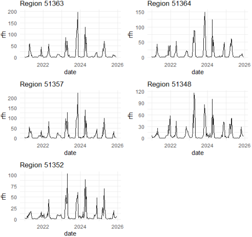
To determine how dekadal rainfall changed over time in the selected regions, time series plots were created.

Figure 1 shows the time series plots of the selected regions. There are uniform trends in the rainfall estimate which show variability in all regions. The series are marked by the low baseline values, with sharp and intermittent spikes, especially around 2023 and 2024, which indicates the impact of common external factors. The highest peaks of 51357 and 51363 are over 200, whereas Regions 51348 and 51352 are lower. The timing and strength are also irregular although there are occasional peaks with similar intervals, which shows there may be weak seasonality.

Download: Download full-size image

Figure 1. Dekadal rainfall series for selected regions.

3.1.2. Transformation

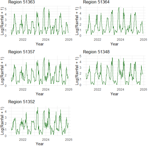
Rainfall time series data were transformed using logarithmic transformation to stabilize the variance and minimize the effect of extreme values. To evaluate the change in the variance stability and the general data behavior, the transformed series were then plotted to visually assess the improvement in the variance stability and general data behavior before model estimation.

Download: Download full-size image

Figure 2. Log-transformed rainfall series.

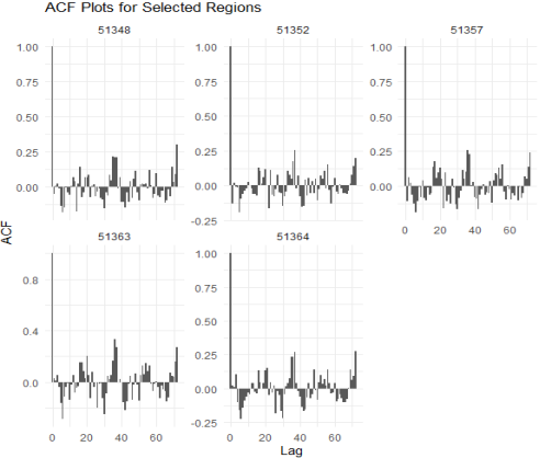
Figure 2 shows the logarithmic transformation of the selected regions. The original series is highly variable with sharp peaks and skewed to the right, which means non-constant variance. After the logarithmic transformation, the extreme values were squeezed, leading to a more symmetric distribution and better variance stability. The change improves the appropriateness of the data to be used in further time series modelling by improving the normality and homoscedasticity assumptions.

3.1.3. Stationarity and Differencing

After the logarithmic transformation, the first order differencing was done to eliminate any residual non-stationarity in the mean. The transformed series were more stable, and the fluctuations were around a constant level indicating that the mean structure had been stabilized sufficiently. To evaluate the stationarity of the rainfall time series in all the regions, the Augmented Dickey Fuller test was used. The preliminary examination of the rainfall data revealed that it had trends and seasonal effects and thus had to be transformed and differenced so as to fit the model. Table 2 shows the results.

Table 2. Augmented Dickey Fuller test results.

Region	ADF Statistic	P-Value	Decision
51363	-8.0116	0.01	Stationary
51364	-7.6915	0.01	Stationary
51357	-7.4921	0.01	Stationary
51348	-7.1506	0.01	Stationary
51352	-7.4230	0.01	Stationary

The results of the ADF test show that each of the regions is stationary following transformation. This is found on the basis of the very negative ADF test statistics, with the range of 8.01 to -7.15, and the p-values of 0.01 of all series. Small p-values are truncated at 0.01 in R, which limits the ability to determine their exact values. However, this limitation does not affect the stationarity conclusion since all reported p-values were below the chosen significance level. The null hypothesis of the presence of a unit root was rejected because the p-values are lower than the standard level of significance of 0.05. This means that the series are stationary and they have a constant time mean. Therefore, the data can be modeled with SARIMA.

3.1.4. Model Identification

Model identification of the regions chosen was done by making use of the ACF plots of the log-transformed and differenced series.

Download: Download full-size image

Figure 3. Autocorrelation Function plots of the selected regions.

The Auto Correlation Function (ACF) plots of the selected regions are shown in figure 3. The general pattern is a low to moderate autocorrelation for the rainfall series, with most of the correlation coefficients near to zero but some positive values occurring on the intermediate and higher lags. This means that there is weak temporal dependence, high rainfall variability and low persistence of rainfall events throughout the regions. There is no evidence of any slow decay in the autocorrelation functions, which means that the transformed and differenced series is stationary and can be used in SARIMA modelling. The high values at the higher lags (particularly regions 51357 and 51363) indicate seasonal dependence, namely annual rainfall cycles. The results are in line with those of previous studies carried out in the Kenya region where loss of coherence of inter-seasonal temporal patterns, weak, but persistent seasonal autocorrelation structures, particularly in arid and semi-arid regions have been reported

[6-11]

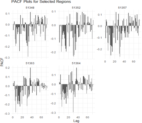
PACF plots were then plotted to determine the appropriate order of the AR component.

Download: Download full-size image

Figure 4. Partial Autocorrelation Function plots of the selected regions.

The Partial Autocorrelation Function (PACF) plots of the selected regions are shown below in Figure 4. The rainfall series are mostly weakly to moderately AR dependent, with positive and negative peaks occurring in the series and decreasing in magnitude with the lag. They are oscillatory patterns reflecting short-term limited persistence, as well as climatic seasonal influences resulting from large-scale climatic processes. Seasonal persistence is relatively stronger in regions 51357 and 51363 with sharper peaks at higher lags, but relatively weaker and higher rainfall variability in other regions. The partial autocorrelations rapidly decrease, indicating that low-order autoregressive components are enough for modelling the rainfall series, which justifies the application of SARIMA models. The results are in line with other studies conducted in Kenya and the rest of East Africa that found that rainfall series are weakly autoregressive, highly variable, and sensitive to the seasonality in the atmosphere, including the Intertropical Convergence Zone (ITCZ) and ENSO

[5-8, 11, 12]

3.1.5. Model Selection

A number of SARIMA models were estimated on the log-transformed rainfall data of each of the selected regions. The patterns in the ACF and PACF plots were used to define the candidate models. The AIC and BIC were used to select models.

Table 3. Candidate SARIMA models.

Region	Model	AIC	BIC	RMSE
51348	SARIMA (1,0,0) (1,1,1)₃₆	288.4007423	300.2521208	0.44705165
51348	SARIMA (0,0,2) (1,1,1)₃₆	288.9737266	303.7879498	0.443114152
51348	SARIMA (2,0,0) (1,1,1)₃₆	290.0999044	304.9141275	0.444693049
51348	SARIMA (1,0,1) (1,1,1)₃₆	290.2065062	305.0207293	0.444917323
51348	SARIMA (2,0,1) (1,1,1)₃₆	290.5298334	308.3069012	0.442953918
51352	SARIMA (1,0,0) (1,1,1)₃₆	292.321006	304.1723845	0.454452909
51352	SARIMA (2,0,0) (1,1,1)₃₆	294.0630678	308.877291	0.453467045
51352	SARIMA (1,0,1) (1,1,1)₃₆	294.0966407	308.9108638	0.453551041
51352	SARIMA (0,0,1) (1,1,1)₃₆	294.2346896	306.0860681	0.459488182
51352	SARIMA (0,0,2) (1,1,1)₃₆	294.3660078	309.180231	0.455599572
51357	SARIMA (1,0,0) (0,1,1)₃₆	320.909477	329.7980109	0.531420296
51357	SARIMA (2,0,0) (0,1,1)₃₆	320.9102977	332.7616762	0.527680834
51357	SARIMA (2,0,0) (1,1,1)₃₆	320.9902052	335.8044284	0.507549281
51357	SARIMA (1,0,0) (1,1,1)₃₆	321.3268755	333.178254	0.512982708
51357	SARIMA (0,0,2) (0,1,1)₃₆	321.326879	333.1782576	0.528440844
51363	SARIMA (1,0,0) (0,1,1)₃₆	282.3509044	291.2394383	0.464209207
51363	SARIMA (1,0,0) (1,1,1)₃₆	282.7458305	294.597209	0.448552228
51363	SARIMA (2,0,0) (0,1,1)₃₆	283.2337881	295.0851666	0.462385335
51363	SARIMA (1,0,1) (0,1,1)₃₆	283.4401762	295.2915547	0.46271469
51363	SARIMA (2,0,0) (1,1,1)₃₆	283.6086186	298.4228418	0.446835138
51364	SARIMA (1,0,0) (1,1,1)₃₆	300.8473512	312.6987298	0.469572074
51364	SARIMA (2,0,0) (1,1,1)₃₆	302.011739	316.8259622	0.468915187
51364	SARIMA (1,0,1) (1,1,1)₃₆	302.1531437	316.9673669	0.469187263
51364	SARIMA (2,0,2) (1,1,1)₃₆	302.7728214	323.5127338	0.468310133
51364	SARIMA (1,0,0) (0,1,1)₃₆	302.80601	311.6945439	0.49848314

The best model based on AIC was chosen as the best model in each region due to its superior performance in forecasting-oriented time series modeling. Results are presented in Table 4.

Table 4. Selected SARIMA models.

Region	Model	AIC	BIC	RMSE
51348	SARIMA (1,0,0) (1,1,1)₃₆	288.4007423	300.2521208	0.44705165
51352	SARIMA (1,0,0) (1,1,1)₃₆	292.321006	304.1723845	0.454452909
51357	SARIMA (1,0,0) (0,1,1)₃₆	320.909477	329.7980109	0.531420296
51363	SARIMA (1,0,0) (0,1,1)₃₆	282.3509044	291.2394383	0.464209207
51364	SARIMA (1,0,0) (1,1,1)₃₆	300.8473512	312.6987298	0.469572074

SARIMA (1,0,0) (1,1,1)₃₆ was found to be best suited for region 51348, 51352 and 51364 in which seasonal AR and MA components were found after applying seasonal differencing. This means that there are periodic seasonal rainfall cycles in these regions. The study conducted by

[13]

, also revealed that the seasonal AR and MA components of SARIMA models were able to describe the seasonality of rainfall in Port Harcourt, Nigeria.

By contrast, SARIMA (1,0,0) (0,1,1)₃₆was found to be the best model for region 51357 and 51363, where only the MA was seasonal was the only component that was significant, suggesting weak seasonal persistence. The inclusion of seasonal MA terms indicates that previous seasonal shocks still have an impact on the current rainfall. Similar findings were reported by

[14]

, who concluded that seasonal MA components are very suitable in capturing the variability of rainfall in Mt. Kenya region.

3.2. Assessing Performance of the Fitted SARIMA Model

3.2.1. Model Diagnostics

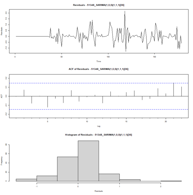
Model diagnostics were performed to investigate the suitability of the fitted SARIMA models. This was done by examining the residual plot, examination of autocorrelation of the residual, and the Ljung box test which was done to determine whether the residual was acting as white noise.

Download: Download full-size image

Figure 5. Residual diagnostics for region 51348.

Download: Download full-size image

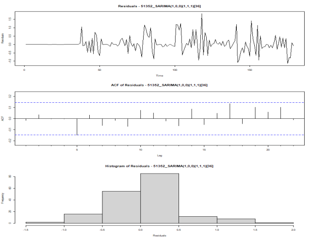
Figure 6. Residual diagnostics for region 51352.

Download: Download full-size image

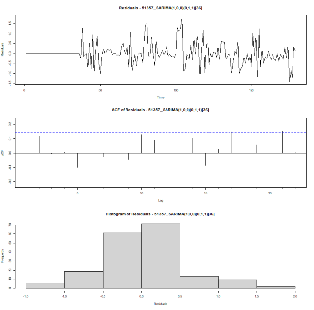
Figure 7. Residual diagnostics for region 51357.

Download: Download full-size image

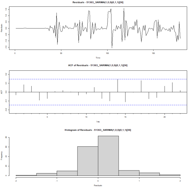
Figure 8. Residual diagnostics for region 51363.

Download: Download full-size image

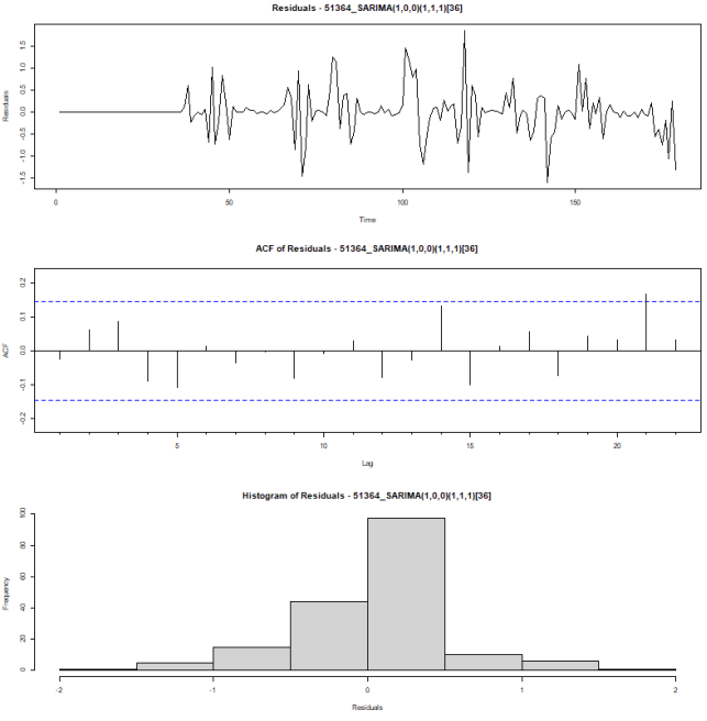
Figure 9. Residual diagnostics for region 51364.

The residual diagnostic plots for the fitted SARIMA models for the selected regions are shown in Figures 5-9. Overall, the residuals are randomly distributed around zero and do not show any obvious pattern or seasonality, thus showing that the models captured the temporal structure of the rainfall series reasonably well. The residual ACF plots indicate that most of the autocorrelation coefficients are within the 95% confidence limits which serve as a test for serial correlation in the residuals, and no strong serial correlation appears. In addition, the residual histograms are roughly symmetric and centered around zero, which is a reasonable assumption of normality. Some isolated residual peaks can be seen but this can be observed in hydroclimatic data as occasional extreme rainfall events and does not imply systematic lack of model skill. The combined diagnostic results indicate that both the fitted SARIMA (1,0,0) (1,1,1)₃₆and SARIMA (1,0,0) (0,1,1)₃₆ models are adequate for representing the dynamics of rainfall and are suitable for forecasting. The results are in line with previous studies that claimed that residuals of well-fitted SARIMA rainfall models are random, have no significant autocorrelation and are close to normality

[13-17]

For the L-Jung test, the null hypothesis is that the distribution of the residuals is independent (there is no autocorrelation), the alternative hypothesis is that there is autocorrelation. The findings are given in Table 5.

Table 5. Ljung-Box Test Results for Residual Diagnostics.

Region	Model ID	LB Statistic	P-Value	Decision
51348	SARIMA (1,0,0) (1,1,1)₃₆	12.2517	0.9071	No autocorrelation
51352	SARIMA (1,0,0) (1,1,1)₃₆	18.2334	0.5720	No autocorrelation
51357	SARIMA (1,0,0) (0,1,1)₃₆	20.7957	0.4092	No autocorrelation
51363	SARIMA (1,0,0) (0,1,1)₃₆	21.5211	0.3671	No autocorrelation
51364	SARIMA (1,0,0) (1,1,1)₃₆	16.8083	0.6654	No autocorrelation

The Ljung–Box test results indicate that all fitted SARIMA models adequately captured the serial dependence in the rainfall series since all p-values were greater than 0.05. Region 51348 exhibited the highest p-value (0.9071), implying very strong residual independence and an excellent model fit. Regions 51352 and 51364 also showed high p-values, confirming that the SARIMA (1,0,0) (1,1,1)₃₆ models successfully removed autocorrelation from the rainfall data. Similarly, Regions 51357 and 51363 fitted with SARIMA (1,0,0) (0,1,1)₃₆ produced non-significant Ljung–Box statistics, indicating that the residuals behaved approximately as white noise. These findings are consistent with

[14]

, who reported that adequate SARIMA rainfall models should yield residuals with insignificant Ljung–Box statistics and no remaining autocorrelation, confirming the reliability of the models for rainfall forecasting.

3.2.2. Model Validation

The fitted SARIMA model’s predictive performance was evaluated by model validation. The data set was separated into a training set and a testing set of which 80 percent of the data was utilized in estimating the model and the rest of the 20 percent of the data was used in validation. Forecasts were then made using the fitted models and compared to the observed values in the test set to evaluate predictive accuracy. To assess the accuracy of the forecasts, the error measures that were used were RMSE, MAE, MAPE and MASE.

Table 6. Forecast Accuracy Measures for the Selected Regions.

Region	RMSE	MAE	MASE	MAPE
51363	0.8490	0.6687	1.1028	121.7738
51364	1.0693	0.9119	1.6095	133.1581
51357	1.2686	1.0586	1.5679	167.2014
51348	1.1896	1.0409	1.8426	1990.7113
51352	1.0117	0.8588	1.4782	133.6153

High MAPE values were observed which may be explained by the nature of rainfall data, which frequently are highly varied and contain very small or zero values. Due to this case, MASE was also considered in this study. The forecast accuracy measures show the differences in the goodness of fit between the fitted SARIMA model for the five regions. The values for region 51363 were the lowest, indicating comparatively better forecast skill. The forecasting performance in regions 51364, 51357 and 51352 were moderate, but the MAE and MASE values for region 51348 were relatively high and therefore achieved relatively larger forecasting errors.

3.3. Forecasting

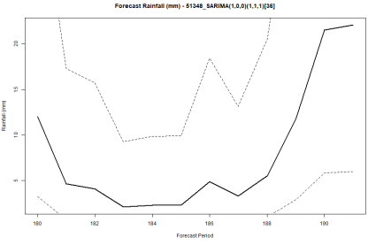
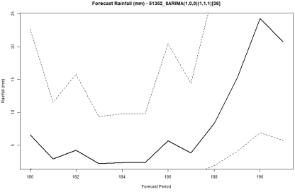
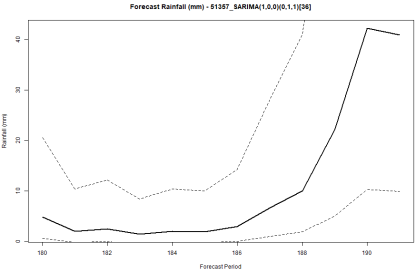
After the estimation and validation of the fitted SARIMA models, prediction was done to test the predictive strength of the models and to forecast future rainfall trends. In this analysis, predictions were made with a horizon of 36 dekads, which is equivalent to one year ahead. The predictions were calculated using the log-transformed rainfall records. Exponential transformation was then applied to the forecasted values to get them back to the original rainfall scale (mm). The trends of the forecasts are graphically presented in the figures below, which illustrate the forecast trajectories for each region together with their corresponding uncertainty bounds. Each plot shows the point forecast (solid line) and the 95% prediction intervals (dashed lines).

Download: Download full-size image

Figure 10. Forecast for region 51348.

The forecast for region 51348 has a "U" shape. At the start of the horizon, rainfall declines followed by several periods of reduced rainfall, and then an abrupt increase in rainfall towards the end of the horizon. The final forecast is above 20 mm, meaning that wetter weather is likely following a long dry spell. The transition is relatively smooth, but there is still significant uncertainty, compared to other regions.

Download: Download full-size image

Figure 11. Forecast for region 51352.

The weather forecast is more complex in region 51352. During the early and middle forecast period rainfall is relatively low, generally less than 5 mm, thus continuing the dry conditions. In the last periods the rate of increase is much higher, with forecast rainfall reaching about 24 mm, then slightly decreasing in the final period. This indicates that intense rainfall will occur in the area for a short time. The prediction intervals are more irregular and wider than in the other regions, reflecting increased uncertainty and a greater historical variability in rainfall in this region being less predictable.

Download: Download full-size image

Figure 12. Forecast for region 51357.

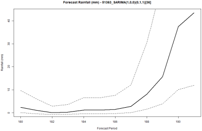
The forecast for region 51357 shows persistently low rainfall throughout the entire forecast period, except for minor variations during the early forecast days. There is a significant rise expected after about period 187. The point forecast is steeply increasing and shows the highest forecast values in all regions, surpassing 40 mm at the end of the forecast period. This means that region 51357 could receive heavy rain during the rainy season. The intervals are also much wider in the case of higher rainfall amounts, indicating greater uncertainty, but the general trend is that there will be a prolonged rainy season.

Download: Download full-size image

Figure 13. Forecast for region 51363.

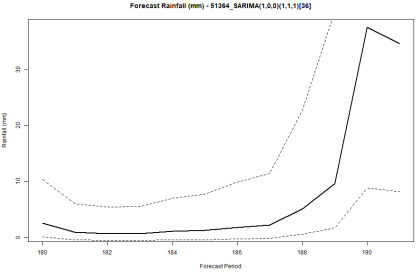
Rainfall is predicted to be below average and fairly consistent over the first few forecast periods in region 51363. The pattern of rising rainfall starts to increase after period 186. As the forecasted period reaches the final period, the amount of rainfall is expected to substantially increase with values above 40 mm for the final forecast periods. This means that the region could experience a lot of rain after a dry season. The increasing confidence intervals suggest that the onset of the rainfall increase is fairly consistent, but the intensity remains uncertain.

Download: Download full-size image

Figure 14. Forecast for region 51364.

The 51364 region forecast shows that the rainfall will be very low for the next few forecast periods with values near zero. This indicates that the dry spell may be prolonged. The model predicts a gradual rise in rainfall starting from forecast period 187, with a steep rise in the last two periods where rainfall is projected to be greater than 30 mm. The pattern is typical of the end of dry season and start of wet season. The prediction intervals are significantly larger at the end of the forecast period, reflecting the greater uncertainty about the size of the rainfall increase.

In all five regions, the forecasts generally indicate a shift from dry conditions to much more precipitation at the end of the forecast period. Regions 51357 and 51363 are expected to see the highest increase, while 51352 faces the highest uncertainty and short-term fluctuations. In general, all regions are expected to have significantly wetter weather in later forecast periods, although the exact magnitude varies and is subject to increasing uncertainty.

4. Conclusion

In conclusion, the study shows that SARIMA models can be used effectively to capture and predict dekadal rainfall variability over the regions under study in Kenya. The obtained results showed that rainfall patterns are highly variable both in space and time and identified SARIMA models were capable of capturing both short-term and seasonal variations. The models generated reasonably accurate forecasts and gave useful information on future rainfall trends despite some limitations arising from the high variability of rainfall. Thus, SARIMA modelling can be useful for supporting agricultural planning, water resource management, and climate risk preparedness, and future studies using longer data sets and including more climatic variables could benefit further forecasting performance.

Abbreviations

ACF	Autocorrelation function
ADF	Augmented Dickey Fuller
AIC	Akaike Information Criteria
AR	Auto Regressive
BIC	Bayesian Information Criterion
CV	Coefficient of Variation
ENSO	El Nino Southern Oscillation
MA	Moving Average
MAE	Mean Absolute Error
MAPE	Mean Absolute Percentage Error
MASE	Mean Absolute Scaled Error
PACF	Partial Autocorrelation Function
RMSE	Root Mean Square Error
SARIMA	Seasonal Autoregressive Integrated Moving Average

Acknowledgments

We wish to express our sincere gratitude to Jacob Chege, Esther Gitei, Kevin Kioria and Kirinyaga University fraternity for their support.

Author Contributions

Linnet Chege: Conceptualization, Data curation, Formal Analysis, Investigation, Methodology, Software, Visualization, Writing – original draft, Writing – review & editing

Peter Gachoki: Project administration, Supervision

Joseph Eyang’an Esekon: Project administration, Supervision

Conflicts of Interest

The authors declare no conflicts of interest.

References

[1]	Palmer, P. I., Wainwright, C. M., Dong, B., Maidment, R. I., Wheeler, K. G., Gedney, N., & Turner, A. G. (2023). Drivers and impacts of Eastern African rainfall variability. Nature Reviews Earth & Environment, 4, 254–270. https://doi.org/10.1038/s43017-023-00397-x
[2]	Alahacoon, N., Edirisinghe, M., Simwanda, M., Perera, E. N. C., Nyirenda, V. R., & Ranagalage, M. (2022). Rainfall variability and trends over the African continent using TAMSAT data (1983–2020): Towards climate change resilience and adaptation. Remote Sensing, 14(1), Article 96. https://doi.org/10.3390/rs14010096
[3]	Alhamshry, A., Fenta, A. A., Yasuda, H., Kimura, R., & Shimizu, K. (2020). Seasonal rainfall variability in Ethiopia and its long-term link to global sea surface temperatures. Water, 12(1), Article 55. https://doi.org/10.3390/w12010055
[4]	Omondi, P., Awange, J. L., Ogallo, L., Okoola, R. A., & Forootan, E. (2012). Decadal rainfall variability modes in observed rainfall records over East Africa and their relations to historical sea surface temperature changes. Journal of Hydrology, 464–465, 140–156. https://doi.org/10.1016/j.jhydrol.2012.07.003
[5]	Filder, T. N., Muraya, M. M., & Mutwiri, R. M. (2019). Application of seasonal autoregressive moving average models to analysis and forecasting of time series monthly rainfall patterns in Embu County, Kenya.
[6]	Mumo, L., Yu, J., & Ayugi, B. (2019). Evaluation of spatiotemporal variability of rainfall over Kenya from 1979 to 2017. Journal of Atmospheric and Solar-Terrestrial Physics, 194, Article 105097. https://doi.org/10.1016/j.jastp.2019.105097
[7]	Langat, P. K., Kumar, L., & Koech, R. (2017). Temporal variability and trends of rainfall and streamflow in Tana River Basin, Kenya. Sustainability, 9(11), Article 1963. https://doi.org/10.3390/su9111963
[8]	Recha, C. W., Shisanya, C., Traore, P. C. S., & Makokha, G. L. (2012). Determination of seasonal rainfall variability, onset and cessation in semi-arid Tharaka District, Kenya. Theoretical and Applied Climatology, 108(3–4), 479–494. https://doi.org/10.1007/s00704-011-0544-3
[9]	Kotikot, S. M., Smithwick, E. A. H., & Greatrex, H. (2024). Observations of enhanced rainfall variability in Kenya, East Africa. Scientific Reports, 14, 63786. https://doi.org/10.1038/s41598-024-63786-2
[10]	Philip Obaigwa Sagero, Chris A. Shisanya, & George L. Makokha (2018). Investigation of rainfall variability over Kenya (1950–2012). Journal of Environmental and Agricultural Sciences, 14, 1–15.
[11]	Ayugi, B., Tan, G., Ullah, W., Boiyo, R., & Ongoma, V. (2019). Inter-comparison of remotely sensed precipitation datasets over Kenya during 1998–2016. Atmospheric Research, 225, 96–109. https://doi.org/10.1016/j.atmosres.2019.03.032
[12]	Samson, T. K., & Aweda, F. O. (2024). Seasonal autoregressive integrated moving average modelling and forecasting of monthly rainfall in selected African stations. Mathematical Modelling of Engineering Problems, 11(1), 159–168. https://doi.org/10.18280/mmep.110117
[13]	Leneenadogo, W. (2021). A comparative study of Fourier series models and seasonal-autoregressive integrated moving average model of rainfall data in Port Harcourt. Asian Journal of Probability and Statistics, 10(3), 36–46.
[14]	Kibunja, H. W., Kihoro, J. M., Orwa, G. O., & Yodah, W. O. (2014). Forecasting precipitation using SARIMA Model: A case study of Mt. Kenya Region.
[15]	Amaefula, C. G. (2021). A SARIMA and adjusted SARIMA models in a seasonal nonstationary time series: Evidence of Enugu monthly rainfall. European Journal of Mathematics and Statistics, 2(1), 13–18. https://doi.org/10.24018/ejmath.2021.2.1.15
[16]	Joshua, K., Herbert, M., & Richard, A. O. (2026). Seasonal ARIMA-based forecasting of monthly rainfall in Kasese District, Uganda.
[17]	Martínez-Acosta, L., Medrano-Barboza, J. P., López-Ramos, Á., et al. (2020). SARIMA approach to generating synthetic monthly rainfall in the Sinú River watershed in Colombia. Atmosphere, 11(6), Article 602. https://doi.org/10.3390/atmos11060602

Cite This Article

Plain Text BibTeX RIS

APA Style

Chege, L., Gachoki, P., Esekon, J. E. (2026). Modelling Dekadal Rainfall Dynamics in Kenyan Subnational Regions Using Sarima Model. American Journal of Theoretical and Applied Statistics, 15(4), 149-163. https://doi.org/10.11648/j.ajtas.20261504.14

Copy | Download

ACS Style

Chege, L.; Gachoki, P.; Esekon, J. E. Modelling Dekadal Rainfall Dynamics in Kenyan Subnational Regions Using Sarima Model. Am. J. Theor. Appl. Stat. 2026, 15(4), 149-163. doi: 10.11648/j.ajtas.20261504.14

Copy | Download

AMA Style

Chege L, Gachoki P, Esekon JE. Modelling Dekadal Rainfall Dynamics in Kenyan Subnational Regions Using Sarima Model. Am J Theor Appl Stat. 2026;15(4):149-163. doi: 10.11648/j.ajtas.20261504.14

Copy | Download

@article{10.11648/j.ajtas.20261504.14,
  author = {Linnet Chege and Peter Gachoki and Joseph Eyang’an Esekon},
  title = {Modelling Dekadal Rainfall Dynamics in Kenyan Subnational Regions Using Sarima Model},
  journal = {American Journal of Theoretical and Applied Statistics},
  volume = {15},
  number = {4},
  pages = {149-163},
  doi = {10.11648/j.ajtas.20261504.14},
  url = {https://doi.org/10.11648/j.ajtas.20261504.14},
  eprint = {https://article.sciencepublishinggroup.com/pdf/10.11648.j.ajtas.20261504.14},
  abstract = {Kenya is very weather sensitive, and the seasonality and variability of rainfall has a significant impact on agricultural productivity, water resource management and food security. Therefore, precise rainfall prediction is a key requirement for climate risk management and decision-making. Most Kenyan rainfall studies have been of monthly and/or annual rainfall, which may not be sensitive enough to the intra-seasonal variability in rainfall seen at dekadal (10-day) time scales. The aim of this study was to model and forecast dekadal rainfall dynamics in selected Sub-national regions of Kenya using Seasonal Autoregressive Integrated Moving Average (SARIMA) models. The quantitative time series research design adopted involved Box–Jenkins methodology with data on dekadal rainfall from 2021 to 2025 from the Humanitarian Data Exchange (HDX). The five regions namely Manyatta, Mbeere North, Igembe Central, Marsabit and Isiolo were chosen for analysis. Data was analyzed by R statistical software. Logarithmic transformation and differencing were used to stabilize the variance and to make the data stationary as verified by the Augmented Dickey–Fuller test. Autocorrelation Function (ACF) and Partial Autocorrelation Function (PACF) were used to identify the candidate SARIMA models, while Akaike Information Criterion (AIC) and Bayesian Information Criterion (BIC) were used to select the models. Model adequacy was checked with residual diagnostics and Ljung–Box test, and the forecasting performance was judged based on RMSE, MAE, MAPE, and MASE. The results showed that SARIMA (1,0,0) (1,1,1)36 was the most suitable model for regions51348,51352, and51364, whereas SARIMA (1,0,0) (0,1,1)36 provided the best fit for regions 51357 and 51363. Residual diagnostics also showed that the models estimated were appropriate to represent the temporal dependence in the rainfall series, as the residuals were in the form of white noise. High MAPE values were observed, which were mostly related to the intermittent nature of the rainfall data, but satisfactory forecasting performance was shown by RMSE, MAE and MASE. Forecasts for the coming year reproduced the observed seasonal rainfall pattern and showed greater uncertainty in the longer-term forecasts. In general, the chosen SARIMA models were successful in modelling dekadal rainfall patterns and can be a valuable tool for agricultural planning, water resource management, and climate risk preparedness for Kenya.},
 year = {2026}
}

Copy | Download

TY  - JOUR
T1  - Modelling Dekadal Rainfall Dynamics in Kenyan Subnational Regions Using Sarima Model
AU  - Linnet Chege
AU  - Peter Gachoki
AU  - Joseph Eyang’an Esekon
Y1  - 2026/08/06
PY  - 2026
N1  - https://doi.org/10.11648/j.ajtas.20261504.14
DO  - 10.11648/j.ajtas.20261504.14
T2  - American Journal of Theoretical and Applied Statistics
JF  - American Journal of Theoretical and Applied Statistics
JO  - American Journal of Theoretical and Applied Statistics
SP  - 149
EP  - 163
PB  - Science Publishing Group
SN  - 2326-9006
UR  - https://doi.org/10.11648/j.ajtas.20261504.14
AB  - Kenya is very weather sensitive, and the seasonality and variability of rainfall has a significant impact on agricultural productivity, water resource management and food security. Therefore, precise rainfall prediction is a key requirement for climate risk management and decision-making. Most Kenyan rainfall studies have been of monthly and/or annual rainfall, which may not be sensitive enough to the intra-seasonal variability in rainfall seen at dekadal (10-day) time scales. The aim of this study was to model and forecast dekadal rainfall dynamics in selected Sub-national regions of Kenya using Seasonal Autoregressive Integrated Moving Average (SARIMA) models. The quantitative time series research design adopted involved Box–Jenkins methodology with data on dekadal rainfall from 2021 to 2025 from the Humanitarian Data Exchange (HDX). The five regions namely Manyatta, Mbeere North, Igembe Central, Marsabit and Isiolo were chosen for analysis. Data was analyzed by R statistical software. Logarithmic transformation and differencing were used to stabilize the variance and to make the data stationary as verified by the Augmented Dickey–Fuller test. Autocorrelation Function (ACF) and Partial Autocorrelation Function (PACF) were used to identify the candidate SARIMA models, while Akaike Information Criterion (AIC) and Bayesian Information Criterion (BIC) were used to select the models. Model adequacy was checked with residual diagnostics and Ljung–Box test, and the forecasting performance was judged based on RMSE, MAE, MAPE, and MASE. The results showed that SARIMA (1,0,0) (1,1,1)36 was the most suitable model for regions51348,51352, and51364, whereas SARIMA (1,0,0) (0,1,1)36 provided the best fit for regions 51357 and 51363. Residual diagnostics also showed that the models estimated were appropriate to represent the temporal dependence in the rainfall series, as the residuals were in the form of white noise. High MAPE values were observed, which were mostly related to the intermittent nature of the rainfall data, but satisfactory forecasting performance was shown by RMSE, MAE and MASE. Forecasts for the coming year reproduced the observed seasonal rainfall pattern and showed greater uncertainty in the longer-term forecasts. In general, the chosen SARIMA models were successful in modelling dekadal rainfall patterns and can be a valuable tool for agricultural planning, water resource management, and climate risk preparedness for Kenya.
VL  - 15
IS  - 4
ER  -

Copy | Download

Author Information

Linnet Chege

Department of Pure & Applied Sciences, Kirinyaga University, Kerugoya, Kenya

Contact Email

http://orcid.org/0009-0003-6580-9687
Peter Gachoki

Department of Pure & Applied Sciences, Kirinyaga University, Kerugoya, Kenya

Contact Email
Joseph Eyang’an Esekon

Department of Pure & Applied Sciences, Kirinyaga University, Kerugoya, Kenya

http://orcid.org/0009-0000-8033-9175

Download PDF

Submit an Article

Plain Text BibTeX RIS

APA Style

Chege, L., Gachoki, P., Esekon, J. E. (2026). Modelling Dekadal Rainfall Dynamics in Kenyan Subnational Regions Using Sarima Model. American Journal of Theoretical and Applied Statistics, 15(4), 149-163. https://doi.org/10.11648/j.ajtas.20261504.14

Copy | Download

ACS Style

Chege, L.; Gachoki, P.; Esekon, J. E. Modelling Dekadal Rainfall Dynamics in Kenyan Subnational Regions Using Sarima Model. Am. J. Theor. Appl. Stat. 2026, 15(4), 149-163. doi: 10.11648/j.ajtas.20261504.14

Copy | Download

AMA Style

Chege L, Gachoki P, Esekon JE. Modelling Dekadal Rainfall Dynamics in Kenyan Subnational Regions Using Sarima Model. Am J Theor Appl Stat. 2026;15(4):149-163. doi: 10.11648/j.ajtas.20261504.14

Copy | Download

@article{10.11648/j.ajtas.20261504.14,
  author = {Linnet Chege and Peter Gachoki and Joseph Eyang’an Esekon},
  title = {Modelling Dekadal Rainfall Dynamics in Kenyan Subnational Regions Using Sarima Model},
  journal = {American Journal of Theoretical and Applied Statistics},
  volume = {15},
  number = {4},
  pages = {149-163},
  doi = {10.11648/j.ajtas.20261504.14},
  url = {https://doi.org/10.11648/j.ajtas.20261504.14},
  eprint = {https://article.sciencepublishinggroup.com/pdf/10.11648.j.ajtas.20261504.14},
  abstract = {Kenya is very weather sensitive, and the seasonality and variability of rainfall has a significant impact on agricultural productivity, water resource management and food security. Therefore, precise rainfall prediction is a key requirement for climate risk management and decision-making. Most Kenyan rainfall studies have been of monthly and/or annual rainfall, which may not be sensitive enough to the intra-seasonal variability in rainfall seen at dekadal (10-day) time scales. The aim of this study was to model and forecast dekadal rainfall dynamics in selected Sub-national regions of Kenya using Seasonal Autoregressive Integrated Moving Average (SARIMA) models. The quantitative time series research design adopted involved Box–Jenkins methodology with data on dekadal rainfall from 2021 to 2025 from the Humanitarian Data Exchange (HDX). The five regions namely Manyatta, Mbeere North, Igembe Central, Marsabit and Isiolo were chosen for analysis. Data was analyzed by R statistical software. Logarithmic transformation and differencing were used to stabilize the variance and to make the data stationary as verified by the Augmented Dickey–Fuller test. Autocorrelation Function (ACF) and Partial Autocorrelation Function (PACF) were used to identify the candidate SARIMA models, while Akaike Information Criterion (AIC) and Bayesian Information Criterion (BIC) were used to select the models. Model adequacy was checked with residual diagnostics and Ljung–Box test, and the forecasting performance was judged based on RMSE, MAE, MAPE, and MASE. The results showed that SARIMA (1,0,0) (1,1,1)36 was the most suitable model for regions51348,51352, and51364, whereas SARIMA (1,0,0) (0,1,1)36 provided the best fit for regions 51357 and 51363. Residual diagnostics also showed that the models estimated were appropriate to represent the temporal dependence in the rainfall series, as the residuals were in the form of white noise. High MAPE values were observed, which were mostly related to the intermittent nature of the rainfall data, but satisfactory forecasting performance was shown by RMSE, MAE and MASE. Forecasts for the coming year reproduced the observed seasonal rainfall pattern and showed greater uncertainty in the longer-term forecasts. In general, the chosen SARIMA models were successful in modelling dekadal rainfall patterns and can be a valuable tool for agricultural planning, water resource management, and climate risk preparedness for Kenya.},
 year = {2026}
}

Copy | Download

TY  - JOUR
T1  - Modelling Dekadal Rainfall Dynamics in Kenyan Subnational Regions Using Sarima Model
AU  - Linnet Chege
AU  - Peter Gachoki
AU  - Joseph Eyang’an Esekon
Y1  - 2026/08/06
PY  - 2026
N1  - https://doi.org/10.11648/j.ajtas.20261504.14
DO  - 10.11648/j.ajtas.20261504.14
T2  - American Journal of Theoretical and Applied Statistics
JF  - American Journal of Theoretical and Applied Statistics
JO  - American Journal of Theoretical and Applied Statistics
SP  - 149
EP  - 163
PB  - Science Publishing Group
SN  - 2326-9006
UR  - https://doi.org/10.11648/j.ajtas.20261504.14
AB  - Kenya is very weather sensitive, and the seasonality and variability of rainfall has a significant impact on agricultural productivity, water resource management and food security. Therefore, precise rainfall prediction is a key requirement for climate risk management and decision-making. Most Kenyan rainfall studies have been of monthly and/or annual rainfall, which may not be sensitive enough to the intra-seasonal variability in rainfall seen at dekadal (10-day) time scales. The aim of this study was to model and forecast dekadal rainfall dynamics in selected Sub-national regions of Kenya using Seasonal Autoregressive Integrated Moving Average (SARIMA) models. The quantitative time series research design adopted involved Box–Jenkins methodology with data on dekadal rainfall from 2021 to 2025 from the Humanitarian Data Exchange (HDX). The five regions namely Manyatta, Mbeere North, Igembe Central, Marsabit and Isiolo were chosen for analysis. Data was analyzed by R statistical software. Logarithmic transformation and differencing were used to stabilize the variance and to make the data stationary as verified by the Augmented Dickey–Fuller test. Autocorrelation Function (ACF) and Partial Autocorrelation Function (PACF) were used to identify the candidate SARIMA models, while Akaike Information Criterion (AIC) and Bayesian Information Criterion (BIC) were used to select the models. Model adequacy was checked with residual diagnostics and Ljung–Box test, and the forecasting performance was judged based on RMSE, MAE, MAPE, and MASE. The results showed that SARIMA (1,0,0) (1,1,1)36 was the most suitable model for regions51348,51352, and51364, whereas SARIMA (1,0,0) (0,1,1)36 provided the best fit for regions 51357 and 51363. Residual diagnostics also showed that the models estimated were appropriate to represent the temporal dependence in the rainfall series, as the residuals were in the form of white noise. High MAPE values were observed, which were mostly related to the intermittent nature of the rainfall data, but satisfactory forecasting performance was shown by RMSE, MAE and MASE. Forecasts for the coming year reproduced the observed seasonal rainfall pattern and showed greater uncertainty in the longer-term forecasts. In general, the chosen SARIMA models were successful in modelling dekadal rainfall patterns and can be a valuable tool for agricultural planning, water resource management, and climate risk preparedness for Kenya.
VL  - 15
IS  - 4
ER  -

Copy | Download