1. Introduction
More than 8% of women suffer from breast cancer in their lifetime. For early detection, various screening programs are held to find its early signs
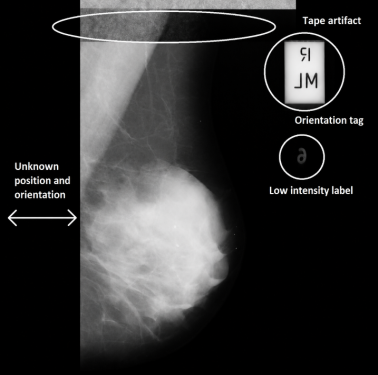
. One of the most widely used methods used in mammography is Computer-aided detection systems. It acts as a tool that enhances the accuracy of human film-reading and classifies signs of breast cancer as malignant or benign. Mammograms often suffer from various kinds of artifact, which are shown in
Figure 1. The publicly available MIAS data set contains scanned film mammograms that contain various artifacts such as, in a few of them, duct tape is present that affects the intensity level of breast tissue while differentiating the cancer tissue from the background on the basis of thresholding. Few of the images in the dataset have unknown positions and orientations that require an accurate position and rotation to all images. Also, few images contain orientation tags as well as low intensity labels, so preprocessing is required for these reasons. For correct segmentation results along with artifact removal, pectoral muscle removal plays a vital role in MLO view of mammograms. The intensity level of the pectoral muscle usually matches the intensity level of abnormalities if present in the mammograms, so sometimes due to the same intensity levels, the results obtained are not correct.
So, this paper focuses on removing all these types of artifacts that hinder the correct segmentation of abnormalities in mammograms. In the past, many methods of preprocessing have been used for initial investigation of the input image. Due to excessive and complex data, a single algorithm is not sufficient, so to handle such issues, we need better methods. Previous work done by researchers has been discussed in this part.
Figure 1. Breast Image showing all types of artifacts.
Various techniques have been presented by many researchers for the detection and removal of pectoral muscles. Shafaq Abbas et. al.
| [2] | S. Abbas, Z. Jalil, A. R. Javed, I. Batool, M. Z. Khan, A. Noorwali, T. R. Gadekallu, and A. Akbar, “BCD-WERT: A novel approach for breast cancer detection using whale optimization based efficient features and extremely randomized tree algorithm,” PeerJ Computer Science, vol. 7, p. e390, 2021,
https://doi.org/10.7717/peerj-cs.390 |
[2]
proposed the BCD-WERT technique for feature selection and classification, which is a combination of the Randomized Tree and Whale Optimization Algorithm. The purpose of WOA is to reduce the dimensionality of the data set to achieve an accurate classification using the relevant features extracted. BCD-WERT achieved an accuracy rate of 99.30%. In order to precisely segment and remove the pectoral muscle, Chen et. al.
| [3] | S. Chen, D. L. Bennett, G. A. Colditz, and S. Jiang, “Pectoral muscle removal in mammogram images: A novel approach for improved accuracy and efficiency,” Cancer Causes & Control, vol. 35, no. 1, pp. 185–191, Jan. 2024,
https://doi.org/10.1007/s10552-023-01781-0 |
[3]
suggested an approach that combined binarization, Canny edge detection, and interpolation techniques. When compared to more conventional tools like Libra, their method produced faster computation and a notable improvement in segmentation accuracy, making it appropriate for real-time applications. Chowdhary et. al.
| [4] | J. Chowdhary, P. Sankaran, and S. Kurup, “A pectoral muscle suppression approach for improved deep learning-based mammogram image analysis,” Biomedical Signal Processing and Control, vol. 112, Part D, p. 108843, Feb. 2026,
https://doi.org/10.1016/j.bspc.2025.108843 |
[4]
gave study on pectoral muscle suppression used a YOLOv8 deep learning model and CLAHE-based preprocessing to incorporate pectoral muscle removal into a full computer-aided diagnosis (CAD) pipeline. Their results demonstrated that the removal of the pectoral muscle greatly enhances the performance of tumor detection, underscoring its significance in automated diagnostic systems. A hybrid approach based on Gaussian Mixture Models (GMM) and line modeling was presented in the Farnoosh et. al.
| [5] | R. Farnoosh and F. Aghagoli, “An innovative computer-based approach for automated preprocessing, enhancement, and pectoral muscle simulation of raw digital mammogram images,” Engineering Applications of Artificial Intelligence, vol. 164, Part A, p. 113215, Jan. 2026,
https://doi.org/10.1016/j.engappai.2025.113215 |
[5]
GMM-based pectoral extraction study. This approach demonstrated the efficacy of combining statistical modeling with geometric constraints by achieving very high segmentation accuracy of about 99% for pectoral muscle removal and mammogram enhancement was presented by Shaikh et. al.
| [6] | S. Shaikh et al., “MammoCare: AI-based mammogram enhancement and pectoral muscle removal system,” in Proc. Int. Conf. on AI in Engineering and Health Sciences (ICAIEHS), Atlantis Press, 2025. |
[6]
in their MammoCare system. Their method emphasizes the shift from standalone algorithms to clinically deployable systems by integrating preprocessing, image enhancement, and visualization. Andrik Rampun et. al.
| [7] | A. Rampun, B. W. Scotney, P. J. Morrow, H. Wang, and J. Winder, “Breast density classification using local quinary patterns with various neighbourhood topologies,” Journal of Imaging, vol. 4, no. 1, p. 14, 2018,
https://doi.org/10.3390/jimaging4010014 |
[7]
investigated a method for density classification in breast images using local Quinary patterns. This method is used to find the texture features of the fibro-glandular region. The Multi-resolution and multi-orientation approach is useful for seeing the neighborhood topologies and correctly finding the most dominant regions. For classification, the SVM classifier is used with promising results. Lazaros Tsochatzidis et. al.
| [8] | L. Tsochatzidis, L. Costaridou, and I. Pratikakis, “Deep learning for breast cancer diagnosis from mammograms—A comparative study,” Journal of Imaging, vol. 5, no. 3, p. 37, 2019,
https://doi.org/10.3390/jimaging5030037 |
[8]
investigated deep convolutional neural networks in the context of the CADx system of breast cancer. These neural networks are trained and evaluated to categorize benign and malignant lesions. Nashid Alam et. al.
| [9] | N. Alam, E. Denton, and R. Zwiggelaar, “Classification of microcalcification clusters in digital mammograms using a stack generalization based classifier,” Journal of Imaging, vol. 5, no. 9, p. 76, 2019. |
[9]
gave a machine learning technique for classification of microcalcifications clusters in mammogram images from 3 databases named MIAS, DDSM and OMI-DB. Initially, the input image is preprocessed using a dynamic wavelet based algorithm followed by number of morphological operations and edge preserving filtering for generating probable microcalcification clusters. After segmenting the MC’s clusters using their proposed morphological operation based segmentation method, three types of characteristic are extracted, named shape, size, and texture. Feature selection is used to extract the most important features, and further classification is performed using 9 classifiers. Chen-Chung Liu et. al.
| [10] | C. Liu, C. Tsai, J. Liu, C. Yu, and S. Yu, “A pectoral muscle segmentation algorithm for digital mammograms using Otsu thresholding and multiple regression analysis,” Computers & Mathematics with Applications, vol. 64, no. 5, pp. 1100–1107, 2012, https://doi.org/10.1016/j.camwa.2012.03.033 |
[10]
gave a method for the removal of pectoral muscle in a mammogram. In this work, initially the position of the pectoral muscle is identified and a rough border is extracted using a combination of the Otsu thresholding scheme and mathematical morphological operations. For exactly segmenting the pectoral muscle, multiple regression analysis is used. The MIAS database is used for experimentation. R. J. Ferrari et. al.
| [11] | R. Ferrari, R. M. Rangayyan, J. E. L. Desautels, R. A. Borges, and A. F. Frere, “Automatic identification of the pectoral muscle in mammograms,” IEEE Transactions on Medical Imaging, vol. 23, no. 2, pp. 232–245, 2004,
https://doi.org/10.1109/TMI.2003.823062 |
[11]
used a method to identify pectoral muscles based on the multiple resolution technique using wavelets. It overcame the limits of the Hough transform. Sze Man Kwok et. al.
| [12] | S. M. Kwok, R. Chandrasekhar, and Y. Attikiouzel, “Automatic pectoral muscle segmentation on mediolateral oblique view mammograms,” IEEE Transactions on Medical Imaging, vol. 23, no. 9, pp. 1129–1140, 2004,
https://doi.org/10.1109/TMI.2004.830529 |
[12]
gave an adaptive in which the cliff detection is utilized iteratively for accurate detection of the pectoral muscle. With prior knowledge of the position of the pectoral muscle, an edge is estimated by straight line, which is later refined using cliff detection. It gave very promising results for all types of dense tissues. Andrik Rampun et. al
| [13] | A. Rampun, K. Linares, P. Morrow, B. Scotney, H. Wang, I. Ocaña, G. Maclair, R. Zwiggelaar, B. M. A. G. Mello, and I. Macia, “Breast pectoral muscle segmentation in mammograms using a modified holistically-nested edge detection network,” Medical Image Analysis, vol. 57, pp. 1–17, 2019,
https://doi.org/10.1016/j.media.2019.06.003 |
[13]
gave an efficient detection method for very complex shapes of pectoral muscles where boundaries were not clear due to certain reasons such as overlapped breast tissues. Saeid Asgari Taghanaki et. al.
| [14] | S. A. Taghanaki, Y. Liu, B. Miles, and G. Hamarneh, “Geometry-based pectoral muscle segmentation from MLO mammogram views,” IEEE Transactions on Biomedical Engineering, vol. 64, no. 11, pp. 2662–2671, 2017,
https://doi.org/10.1109/TBME.2017.2652371 |
[14]
gave a geometry based pectoral muscle detecting technique that worked for all types of tissue densities. This method gave good results for around 870 images of different tissue density classes. Dilovan Asaad Zebari et. al
| [15] | D. A. Zehari, D. Q. Zeebaree, A. M. Abdulazeez, H. Haron, and H. N. A. Hamed, “Improved threshold-based and trainable fully automated segmentation for breast cancer boundary and pectoral muscle in mammogram images,” IEEE Access, vol. 8, pp. 203097–203116, 2020, https://doi.org/10.1109/ACCESS.2020.3035989 |
[15]
built a unique method to separate the pectoral muscle from the breast region in which initially the breast region is separated from all background artifacts and then HOG (histogram of oriented gradient) features are extracted from the breast part and the pectoral muscle part both. This model utilized 25 mammogram samples to train the neural network, which is used further to testing 3 databases consisting of a total of 622 MLO mammograms. Mehdi Hassan et. al.
| [16] | M. Hassan, A. Chaudhry, A. Khan, M. Iftikhar, and J. Kim, “Medical image segmentation employing information gain and fuzzy C-means algorithm,” in Proc. Int. Conf. on Open Source Systems and Technologies (ICOSST), 2013, pp. 34–39,
https://doi.org/10.1109/ICOSST.2013.6720602 |
[16]
developed a robust clustering method named information gain based FCM that overcomes the shortcomings of traditional FCM. This method is applied to artery ultrasound images for segmenting the images and gave very good results in terms of quantitative measures. Md Shamim Hossain
| [17] | M. Hossain, “Microcalcification segmentation using modified U-Net segmentation network from mammogram images,” Journal of King Saud University – Computer and Information Sciences, 2019, https://doi.org/10.1016/j.jksuci.2019.10.014 |
[17]
worked on an automated system for the detection of calcifications in mammograms. The input image is enhanced using the Laplacian filter and the region of interest is extracted using pixel-wise clustering K-means. The pixels are labeled into two different classes named breast region and pectoral muscle region based on similar intensities and gradient weights. After removing the pectoral muscle part, the suspicious region containing microcalcifications is extracted by splitting the whole image to identical regions and for each region histogram is calculated. The histograms with high intensity will represent the bright spots. Optimal threshold is determined using Fuzzy C-mean clustering method. So in this way, few of the patches containing microcalcifications are separated from background region and are used to train the U-net segmentation network. This network is used for automatically segmenting the area containing microcalcifications. Mario Mustra et. al.
has removed the artifacts before moving on to pectoral muscle removal. The first step in preprocessing is breast alignment in which straight line is detected using sobel edge detection filter and the longest edge detected is considered as breast tissue edge and depending on the its positioned it is aligned to top-left corner using hough transform. For pectoral muscle detection in low contrast areas combination of CLAHE algorithm for contrast enhancement, morphological operations to remove background noises and cubic polynomial functions are applied on ROI. Indra Kanta Maitra et. al.
| [19] | I. Maitra, S. Nag, and S. Bandyopadhyay, “Technique for preprocessing of digital mammogram,” Computer Methods and Programs in Biomedicine, vol. 107, no. 2, pp. 175–188, 2012,
https://doi.org/10.1016/j.cmpb.2011.08.017 |
[19]
gave good results compared to other segmentation methods. They used CLAHE method for enhancement as initial step and for pectoral muscle detection, a rectangle is marked containing pectoral muscle and seeded region growing algorithm is used to isolate it. Trinthi Thu Hah et. al.
| [20] | T. Hah, J. Kim, and S. Choi, “White matter hyperintensities extraction based T2-FLAIR MRI using non-local means filter and nearest neighbor algorithm,” in Proc. Int. Conf. on IT Convergence and Security (ICITCS), 2014, pp. 1–4,
https://doi.org/10.1109/ICITCS.2014.7021830 |
[20]
gave a segmentation technique for extracting the brain image and classified them into 3 classes named ROI, non-ROI and background area. For carrying out this segmentation, two steps are followed, initially the brain matter is removed out of cranium using combination of k-mean clustering and morphological operations and in the other phase non-local mean filter and nearest neighbor algorithm is applied for denoising and diving brain image into 3 classes.
The main contributions of this work are summed up:
1) An enhanced method namely IGFCM (information gain based fcm) combines fuzzy C-mean (fcm) and neutroscopic L-means (nlm) methods for correctly extracting the pectoral muscle.
2) The proposed methodology is tested and validated on different mammographic images in the MIAS database
3) The obtained results are similar to the marked ones by an expert radiologist.
4) On the basis of different metrics the results obtained are compared with the marked ones.
2. Preprocessing
Before any analysis of mammography can begin, image preprocessing must be done. Image preprocessing will ensure that all areas of the image that are not breast tissue have been removed from the image and, thus, will allow for further evaluation of the breast. In this process, any remaining parts after artifact and background removal have been isolated from the original image to allow for future assessment of these areas for reasons of detecting an abnormality. This procedure usually involves the removal of any extraneous marks or noise around the imaged area, locating and delineating the boundary of the breast, removing the area of the pectoral muscle, and enhancing the breast tissue itself to create a more precise image with less extraneous items to distract the reader from the relevant features of the breast. Preprocessing is how you take out any distractions from the mammogram so you only see the important information and not any extraneous items. Preprocessing also reduces noise in the mammogram image; excessive noise may result in false positive results on mammogram segmentation and detection.
In most MLO views, the main area of density is pectoral muscle and can affect the image processing results. For example, the intensity based methods may be misperforming in differentiating dense structures such as the fibro-glandular disk and small doubtful weights, since the intensity of pectoral muscle pixels is roughly same as dense tissues intensity of the image. The pectoral muscle may have an even significant need to find the location of unrequired lymph nodes, which is a single manifestation of obscene breast carcinoma, with local information on the borders of the pectoral muscle along with an internal examination of its area
| [8] | L. Tsochatzidis, L. Costaridou, and I. Pratikakis, “Deep learning for breast cancer diagnosis from mammograms—A comparative study,” Journal of Imaging, vol. 5, no. 3, p. 37, 2019,
https://doi.org/10.3390/jimaging5030037 |
[8]
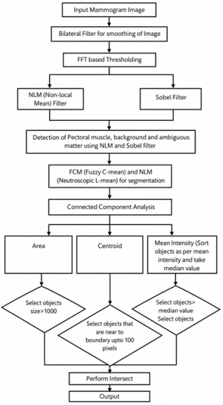
. So it became very essential to do this as it causes a lot of variations in the final results. This work is carried out step by step as shown in
Figure 2 and few modifications wherever required are done to obtain desirable results. Following sections will describe each of the steps including usage of bilateral filters, thresholding and other filters that are carried out for performing the preprocessing of the input image and its requirement.
2.1. Bilateral Filters
Bilateral filters are non-linear filters that retain the edge and have noise reduction properties. Through this filter, the noise content can be filtered without overblurring the image to maintain the clarity of the film. The principal reasoning in background of bilateral filter is that not even when pixels are found in adjacent places, it is assumed to be close together regardless of their overlap in size. The benefit of a two-sided filter relative to traditional Gaussian filter is to use the pressure shifts in bilateral filter to preserve the edges of the image. In a particular neighborhood, it determines the weighted pixel number. A weighted method is used for substitution of the pixel value for adjacent pixel
.
(1)
It works by taking a weighted average of nearby pixels, where p and q denotes the pixel coordinates, S denotes how the intensity values are distributed in space of Ix(x), gs is spatial Gaussian function that gives less importance to pixels that are farther away, fr is a Gaussian range that minimizes the effect of pixel q with an intensity value different from Ip. Further, Wp is the normalization component to be determined using the following equation;
(2)
In this case p and q are pixel coordinates, gs represents the co-ordinate differences smoothing space kernel, fr is the smoothing pressure differences set kernel and S represents the Ix(x) space field.
2.2. FFT Based Thresholding
Fourier analysis was a novel thing that statisticians across the globe had to ’adjust’ for over a decade. In essence, Fourier Transformation’s large contribution states that all functions can be expressed through a weighing function as integral of the sines or cosines. It works for all kinds of complicated components, as long as it includes a certain mild math, it can be thus represented. The feature could be recreated fully via an inversion process, which is expressed in a Fourier transformation
.
The fast Fourier transform termed as F (u) for only one variable can be described by using function f (x) as
:
Here in the above equation j = . In the opposite manner the inverse Fourier transform can be represented as:
(4)
Figure 2. Proposed Methodology.
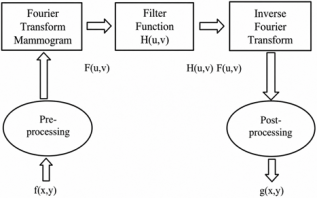
The above two equations make the pair of Fourier transforms that can be used without any loss of the information shown in
Figure 3.
Figure 3. Filtering steps in frequency domain.
2.3. Non-local Means Filter
This filter
| [23] | M. Haque and M. Uddin, “Accelerating fast Fourier transformation for image processing using graphics processing unit,” Journal of Emerging Trends in Computing and Information Sciences, vol. 2, no. 8, pp. 367–375, 2011. |
[23]
is used to smooth the extracted image obtained from the previous stage. Every pixel’s current value is modified on the basis of the comparison of a specified square pixel region with the other pixels. The non-local method process is the following. The new value of the pixels I of image with v = {v
i: gray value of pixel i: iϵI} using a non-local mean filter approach by calculating each pixel’s value as the weighted combination of contributions from many other pixels across the image, is determined as pixel I of image:
The more comparable geometrical form and the greater weighted interest in pixel districts;
(6)
Value of Zi constant can be calculated as:
(7)
The upgrade method for Gray values is based on square area’s geometric picture environment. Noises are filtered with this filter, the image is smoothed and the shape of the image is retained as well.
2.4. Sobel Filter
The edge detector is a basic method that is used in image detection and extraction, primarily to identify and remove optical image points at which the luminosity of the image varies significantly and discontinuities are detected.
| [24] | A. Buades, B. Coll, and J. M. Morel, “A non-local algorithm for image denoising,” in Proc. IEEE Computer Society Conf. on Computer Vision and Pattern Recognition (CVPR), vol. 2, 2005, pp. 60–65, https://doi.org/10.1109/CVPR.2005.38 |
[24]
Sobel edge detection algorithm is based on the process of gradient edge detection that detects the edges of images by horizontal and vertical masks. The transposition of alternative is one sheet. Let [P], the horizontal and vertical mask is merged into a sub-window of 3 to 3 for supplying the horizontal gradient G
x and G
y vertical gradient.
The kernels are meant to reverse vertically, horizontally connected edges of the pixel grid as far as possible. The G
x kernel represents horizontal orientation and the G
y is perpendicular to each other. For both the direction, different gradient components are obtained for the image. The gradient components are obtained by a discrete transfer of the kernels to the input image for vertical and horizontal orientation. By integrating the individual gradient of both orientations, absolute gradient magnitude value is calculated. The sum value of the gradient is
| [25] | R. Menaka, S. Janarthanan, and K. Deeba, “FPGA implementation of low power and high speed image edge detection algorithm,” Microprocessors and Microsystems, vol. 75, p. 103053, 2020, https://doi.org/10.1016/j.micpro.2020.103053 |
[25]
:
(9)
(10)
As shown in below equation, this can be approximated for the absolute magnitude estimation more easily:
In comparison to the pixel grid, the spatial gradient determined by orientation angle is shown as
| [7] | A. Rampun, B. W. Scotney, P. J. Morrow, H. Wang, and J. Winder, “Breast density classification using local quinary patterns with various neighbourhood topologies,” Journal of Imaging, vol. 4, no. 1, p. 14, 2018,
https://doi.org/10.3390/jimaging4010014 |
[7]
:
2.5. Fuzzy-c-means (FCM) Clustering
The solution suggested is an extension of the standard FCM algorithm as stated earlier. This section then discusses first the FCM algorithm and its equations, and then explains in detail the suggested IGFCM.
2.5.1. Traditional Fuzzy C-means Clustering
It is one of the most popular segmentation algorithms. This varies from traditional k mean clustering in that the clustering mechanism incorporates fluid knowledge. The pixel category is allocated to a specific cluster depending on the fluidity of their membership. The following cost function shall be reduced by FCM:
(13)
In the above equation, uij shows the pixel’s membership for xj to the ith element of cluster. vi denotes centroid of cluster, m is the constant variable also called fuzzy index usually with value 2 and total number of clusters are represented by C. By updating the clusters center, the cost function is minimized iteratively. For update fuzzy membership functions and cluster centers, the following mathematical formulas are used:
(14)
where,
(15)
2.5.2. The Proposed Information Gain Based FCM
Classical FCM algorithms are highly noise sensitive and can result in non- homogeneous clusters. The basic FCM structure is expanded with the use of information gain methods to better solve the noise problem. In his pioneering work on information theory
,
Claude Shannon coined the concept of entropy. Information gain is used to quantify how well a specific attribute contributes to the segmentation process and to assess the uncertainty surrounding a random variable. The input image is first segmented using the traditional FCM technique in the suggested IGFCM algorithm, but only for a small number of iterations. By examining the nearby pixels, entropy and information gain are computed for each pixel in its local neighborhood. The suggested method outperforms other approaches when a 5x5 window is used, according to experimental results, and the window size is chosen empirically.
After that, each pixel’s fuzzy membership values are refined by switching them. The information gain ranking of the corresponding clusters dictates the order in which these membership values are switched. The FCM is focused on current member values and newly determined centroids. This cycle persists until the gap between clusters centroid value decreases below a certain threshold or the maximum number of generations. In one step by step algorithm, the procedure is explained as follows:
Proposed Algorithm
Phase I: -
Carried on the input image, the FCM segmentation.
1) First Calculate for every (k, n), vkn (first cluster centroids)
2) Compute ujk for all (j, k) (values of initial fuzzy membership)
Phase I ends with three iterations of the FCM algorithm segmenting the image. Phase I output is supplied further to phase II for computation.
Phase II: -
1) Iterate through the segmented image of FCM by using a 5×5 window.
2) Calculation of probability for each class using below equation:
In the above equation, ni represents the all no. of pixels that belongs to class i in window. N represents the total pixels within the specified window size.
Calculate entropy for every class using the following formula:
(17)
Now use the following formula to determine the entropy of two classes:
(18)
Calculate EI (expected information) using the below equation:
(19)
Calculate Information Gain for each class by using the below equation:
(20)
Calculate;
(21)
Update the value of by using the below expression:
(22)
In the above equation, IG represents the information set of gain values for entire classes and rank of number i is returned by the rank (IG, i) from the set of IG.
Update v
kn from equation (
3) by using the
for every n pixel.
Use the variables vkn and ujk to do the iteration of FCM.
Repeat all of the above steps before you have reached the stop criteria. The stopping criterion is described as if the maximum difference between the cluster centers in two consecutive iterations or if a certain number of iterations of Phase II are completed is below some random threshold. The defuzzification of ujk ultimately produces the final segmented image generated by the IGFCM algorithm.
2.6. Connected Component Analysis (CCA)
In this case, it is done to mark the different connected components using the connected component labeling procedure. Connected labeling of components is essential in many applications for image processing. For such algorithms
| [27] | N. Vishwanath, S. Somasundaram, M. Ravi, and N. Nallaperumal, “Connected component analysis for Indian license plate infra-red and color image character segmentation,” in Proc. IEEE Int. Conf. on Computational Intelligence and Computing Research (ICCIC), 2012, pp. 1–4,
https://doi.org/10.1109/ICCIC.2012.6510323 |
[27]
, there are typically following steps:
1) The first step is to binarize the input image by thresholding technique. Binarization is a process of classifying an image into two different parts.
2) After that, connected component labeling is performed so that each separate region in the image is assigned its own unique label.
3) A variety of characteristics of the body identified by the region (for example, area, center of gravity, bounding chamber etc.) will be analyzed (based on their label).
The characteristics of concern for each component or area must be taken during the study of its related components in order to obtain a single pass streaming algorithm. It eliminates the need to create a labelled picture and guarantees that the second, rebelling transfer is carried out. Fusion and re-labeling must also be carried out on a fly in order to ensure reliable results. In the proposed work, we used three properties of CCA namely Area, Centroid and mean intensities of the image that represents the particular properties of the image obtained after the connected component analysis.
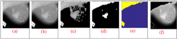
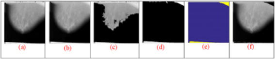
The proposed algorithm for pectoral muscle removal does not use any training set so we can say that all images are in test set only. Results of few images from MIAS database such as mdb206, mdb009 are shown below in
Figure 4(a-f) and
Figure 5(a-f) respectively.
Figure 4. Output of each step of proposed algorithm, (a) Original image mdb206, (b) Bilateral filtered image, (c) Image after FFT based filtering and thresholding, (d) Result after modified Fuzzy C-mean clustering, (e) Segmentation of pectoral muscle logo and other objects, (f) Region of interest left after exclusion of pectoral muscle, label, etc.
Figure 5. Output of each step of proposed algorithm, (a) Original image mdb009, (b) Bilateral filtered image, (c) Image after FFT based filtering and thresholding, (d) Result after modified Fuzzy C-mean clustering, (e) Segmentation of pectoral muscle logo and other objects, (f) Region of interest left after exclusion of pectoral muscle, label, etc.
3. Results and Discussion
Compared to digital images, scanned images typically contain a higher level of noise and unwanted artifacts. The MIAS database consists of scanned film mammograms, which makes pre-processing an essential step before analysis. Several types of artifacts
have been reported in the literature, including: (1) the presence of duct tape, which lowers the intensity of breast tissue and makes simple threshold-based segmentation ineffective; (2) variations in breast position and orientation, requiring proper image registration to ensure consistent alignment across all images; (3) orientation markers; (4) low-intensity labels; and (5) general scanning-related distortions.
The source of the mammograms used in this work is the MIAS database
. The work is performed using MATLAB 2015. Each image in MIAS database is 1024 by 1024 pixels in size. The database includes images from 161 patients, covering both left and right breasts, resulting in a total of 322 mammograms. These images are categorized into three groups: normal, benign, and malignant. Specifically, the dataset contains 208 normal images, 63 benign cases, and 51 malignant (cancerous) cases. Among the 322 mammograms, 150 images include visible pectoral muscle.
The performance of the proposed approach is evaluated using several quantitative metrics, including Hausdorff Distance (HD), Mean Error (ME1), Relative Foreground Area Error (RFAE), Misclassification Rate (ME2), Extraction Error Rate (EER), and Region Non-Uniformity (RNU). The values of the mentioned parameters vary between 0 and 1 where 0 value points to perfectly segmented case. Following is the explanation of each parameter:
Mean Error:
(24)
where m denotes the total pectoral muscle pixels, (xm, ym) are the coordinates of pectoral muscle that is manually marked by radiologist, and (xd, yd) are the coordinates of pectoral muscle that is detected. If the mean error is near to zero that means the marked and detected pectoral muscle are nearly same.
Misclassification Error: It computes the error rate of an algorithm defined as:
(25)
where MTP is the true positive area, MTN is the true negative area, MFP is the false positive area and MFN is the false negative area.
Relative Foreground Area Error: It is used to compute the incorrectness between the manually marked and detected pectoral muscle defined as:
(26)
where MTP + MFN represents the manual marking of pectoral muscle while MFP +MTP represents the detected pectoral muscle.
Extraction Error Rate: It is used to find the non-performance rate of an algorithm and is defined as:
(27)
Region Non-Uniformity: It is used to find a distinct quality in the detected and the manually marked pectoral muscle defined as:
(28)
Hausdorff distance: This is used to determine the likeness in shape between the manually marked area (Am) the detected part defined as:
(29)
where |Am| is the number of pixels in manually marked pectoral muscle Am.dis(a,Ad) is the distance between pixel a and detected pectoral muscle area i.e. defined as:
(30)
where dis(a,b) is the Euclidean distance form pixel a to b.
To demonstrate the performance of the algorithm proposed for pectoral muscle removal we have compared the obtained results with related schemes. Two schemes are used for comparison out of which first one is Ferrar et. al.
| [11] | R. Ferrari, R. M. Rangayyan, J. E. L. Desautels, R. A. Borges, and A. F. Frere, “Automatic identification of the pectoral muscle in mammograms,” IEEE Transactions on Medical Imaging, vol. 23, no. 2, pp. 232–245, 2004,
https://doi.org/10.1109/TMI.2003.823062 |
[11]
and the other one is Chen-Chung Liu et. al.
| [10] | C. Liu, C. Tsai, J. Liu, C. Yu, and S. Yu, “A pectoral muscle segmentation algorithm for digital mammograms using Otsu thresholding and multiple regression analysis,” Computers & Mathematics with Applications, vol. 64, no. 5, pp. 1100–1107, 2012, https://doi.org/10.1016/j.camwa.2012.03.033 |
[10]
. The comparison results obtained on MIAS database are all explained in
Figure 6,
Table 1,
Table 2 and
Table 3.
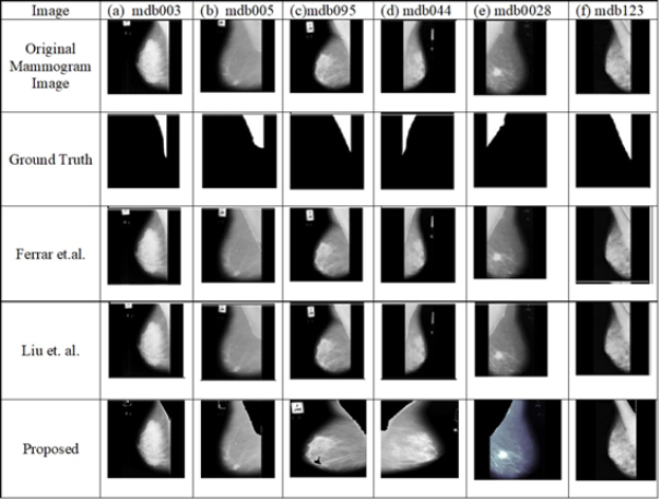
Figure 6 presents the visual results obtained from all the existing algorithms and proposed one on six mammograms that contains pectoral muscles. In
Figure 6 the first row presents the original mammogram images from the MIAS database that were selected for the experiments. The second row displays the corresponding ground truth images, where the pectoral muscle region has been manually outlined by an expert radiologist. The third and fourth rows illustrate the results produced by two authors Ferraret. al.
| [11] | R. Ferrari, R. M. Rangayyan, J. E. L. Desautels, R. A. Borges, and A. F. Frere, “Automatic identification of the pectoral muscle in mammograms,” IEEE Transactions on Medical Imaging, vol. 23, no. 2, pp. 232–245, 2004,
https://doi.org/10.1109/TMI.2003.823062 |
[11]
and Chen-Chung Liu et. al
| [10] | C. Liu, C. Tsai, J. Liu, C. Yu, and S. Yu, “A pectoral muscle segmentation algorithm for digital mammograms using Otsu thresholding and multiple regression analysis,” Computers & Mathematics with Applications, vol. 64, no. 5, pp. 1100–1107, 2012, https://doi.org/10.1016/j.camwa.2012.03.033 |
[10]
respectively. The fifth row corresponds to our obtained results from our proposed algorithm.
The parameter values obtained for all six mammogram images are briefed in
Table 1,
Table 2 and
Table 3. It can be seen that the results from proposed scheme have lower values that means they are near to perfect segmentation of pectoral muscle.
The range and average of all the parameters for 150 cases are shown in
Table 4 and
Table 5. All the six parameters have a much larger ranges for the proposed method as compared to the previous methods. So we can say that this proposed method gives very reliable results for pectoral muscle detection for a mammogram image.
Figure 6. Results obtained by Ferrar et. al., Liu et. al. and the proposed schemes on six mammogram images from MIAS database.
Table 1.
Mean error (me1) and misclassification error (me2) parameter values obtained by using ferrar et al. | [11] | R. Ferrari, R. M. Rangayyan, J. E. L. Desautels, R. A. Borges, and A. F. Frere, “Automatic identification of the pectoral muscle in mammograms,” IEEE Transactions on Medical Imaging, vol. 23, no. 2, pp. 232–245, 2004,
https://doi.org/10.1109/TMI.2003.823062 |
| [10] | C. Liu, C. Tsai, J. Liu, C. Yu, and S. Yu, “A pectoral muscle segmentation algorithm for digital mammograms using Otsu thresholding and multiple regression analysis,” Computers & Mathematics with Applications, vol. 64, no. 5, pp. 1100–1107, 2012, https://doi.org/10.1016/j.camwa.2012.03.033 |
Image | ME1 | ME2 |
Author1 | [11] | R. Ferrari, R. M. Rangayyan, J. E. L. Desautels, R. A. Borges, and A. F. Frere, “Automatic identification of the pectoral muscle in mammograms,” IEEE Transactions on Medical Imaging, vol. 23, no. 2, pp. 232–245, 2004,
https://doi.org/10.1109/TMI.2003.823062 |
[11] | Author2 | [10] | C. Liu, C. Tsai, J. Liu, C. Yu, and S. Yu, “A pectoral muscle segmentation algorithm for digital mammograms using Otsu thresholding and multiple regression analysis,” Computers & Mathematics with Applications, vol. 64, no. 5, pp. 1100–1107, 2012, https://doi.org/10.1016/j.camwa.2012.03.033 |
[10] | Proposed Method | Author1 | [11] | R. Ferrari, R. M. Rangayyan, J. E. L. Desautels, R. A. Borges, and A. F. Frere, “Automatic identification of the pectoral muscle in mammograms,” IEEE Transactions on Medical Imaging, vol. 23, no. 2, pp. 232–245, 2004,
https://doi.org/10.1109/TMI.2003.823062 |
[11] | Author2 | [10] | C. Liu, C. Tsai, J. Liu, C. Yu, and S. Yu, “A pectoral muscle segmentation algorithm for digital mammograms using Otsu thresholding and multiple regression analysis,” Computers & Mathematics with Applications, vol. 64, no. 5, pp. 1100–1107, 2012, https://doi.org/10.1016/j.camwa.2012.03.033 |
[10] | Proposed Method |
Mdb003 | 1.01 | 0.86 | 0.68 | 0.43 | 0.40 | 0.39 |
Mdb005 | 0.34 | 0.18 | 0.14 | 0.04 | 0.02 | 0.02 |
Mdb028 | 1.63 | 0.70 | 0.68 | 0.22 | 0.08 | 0.07 |
Mdb044 | 0.91 | 0.68 | 0.59 | 0.39 | 0.08 | 0.08 |
Mdb095 | 0.13 | 0.11 | 0.11 | 0.00 | 0.00 | 0.00 |
Mdb123 | 20.96 | 20.70 | 20.30 | 0.79 | 0.72 | 0.65 |
Table 2.
Relative Foreground Area Error (RFAE) and Extraction Error Rate (EER) parameter values obtained by using Ferrar et al. | [11] | R. Ferrari, R. M. Rangayyan, J. E. L. Desautels, R. A. Borges, and A. F. Frere, “Automatic identification of the pectoral muscle in mammograms,” IEEE Transactions on Medical Imaging, vol. 23, no. 2, pp. 232–245, 2004,
https://doi.org/10.1109/TMI.2003.823062 |
| [10] | C. Liu, C. Tsai, J. Liu, C. Yu, and S. Yu, “A pectoral muscle segmentation algorithm for digital mammograms using Otsu thresholding and multiple regression analysis,” Computers & Mathematics with Applications, vol. 64, no. 5, pp. 1100–1107, 2012, https://doi.org/10.1016/j.camwa.2012.03.033 |
Image | RFAE | EER |
Author1 | [11] | R. Ferrari, R. M. Rangayyan, J. E. L. Desautels, R. A. Borges, and A. F. Frere, “Automatic identification of the pectoral muscle in mammograms,” IEEE Transactions on Medical Imaging, vol. 23, no. 2, pp. 232–245, 2004,
https://doi.org/10.1109/TMI.2003.823062 |
[11] | Author2 | [10] | C. Liu, C. Tsai, J. Liu, C. Yu, and S. Yu, “A pectoral muscle segmentation algorithm for digital mammograms using Otsu thresholding and multiple regression analysis,” Computers & Mathematics with Applications, vol. 64, no. 5, pp. 1100–1107, 2012, https://doi.org/10.1016/j.camwa.2012.03.033 |
[10] | Proposed Method | Author1 | [11] | R. Ferrari, R. M. Rangayyan, J. E. L. Desautels, R. A. Borges, and A. F. Frere, “Automatic identification of the pectoral muscle in mammograms,” IEEE Transactions on Medical Imaging, vol. 23, no. 2, pp. 232–245, 2004,
https://doi.org/10.1109/TMI.2003.823062 |
[11] | Author2 | [10] | C. Liu, C. Tsai, J. Liu, C. Yu, and S. Yu, “A pectoral muscle segmentation algorithm for digital mammograms using Otsu thresholding and multiple regression analysis,” Computers & Mathematics with Applications, vol. 64, no. 5, pp. 1100–1107, 2012, https://doi.org/10.1016/j.camwa.2012.03.033 |
[10] | Proposed Method |
Mdb003 | 0.08 | 0.07 | 0.06 | 0.06 | 0.06 | 0.06 |
Mdb005 | 0.00 | 0.00 | 0.00 | 0.01 | 0.01 | 0.01 |
Mdb028 | 0.09 | 0.01 | 0.01 | 0.03 | 0.01 | 0.01 |
Mdb044 | 0.06 | 0.01 | 0.01 | 0.05 | 0.01 | 0.00 |
Mdb095 | 0.00 | 0.00 | 0.00 | 0.01 | 0.00 | 0.00 |
Mdb123 | 0.09 | 0.08 | 0.07 | 0.57 | 0.52 | 0.51 |
Table 3.
Region non-uniformity (rnu) and hausdorff distance (hd) parameter values obtained by using ferrar et al. | [11] | R. Ferrari, R. M. Rangayyan, J. E. L. Desautels, R. A. Borges, and A. F. Frere, “Automatic identification of the pectoral muscle in mammograms,” IEEE Transactions on Medical Imaging, vol. 23, no. 2, pp. 232–245, 2004,
https://doi.org/10.1109/TMI.2003.823062 |
| [10] | C. Liu, C. Tsai, J. Liu, C. Yu, and S. Yu, “A pectoral muscle segmentation algorithm for digital mammograms using Otsu thresholding and multiple regression analysis,” Computers & Mathematics with Applications, vol. 64, no. 5, pp. 1100–1107, 2012, https://doi.org/10.1016/j.camwa.2012.03.033 |
Image | RNU | HD |
Author1 | [11] | R. Ferrari, R. M. Rangayyan, J. E. L. Desautels, R. A. Borges, and A. F. Frere, “Automatic identification of the pectoral muscle in mammograms,” IEEE Transactions on Medical Imaging, vol. 23, no. 2, pp. 232–245, 2004,
https://doi.org/10.1109/TMI.2003.823062 |
[11] | Author2 | [10] | C. Liu, C. Tsai, J. Liu, C. Yu, and S. Yu, “A pectoral muscle segmentation algorithm for digital mammograms using Otsu thresholding and multiple regression analysis,” Computers & Mathematics with Applications, vol. 64, no. 5, pp. 1100–1107, 2012, https://doi.org/10.1016/j.camwa.2012.03.033 |
[10] | Proposed Method | Author1 | [11] | R. Ferrari, R. M. Rangayyan, J. E. L. Desautels, R. A. Borges, and A. F. Frere, “Automatic identification of the pectoral muscle in mammograms,” IEEE Transactions on Medical Imaging, vol. 23, no. 2, pp. 232–245, 2004,
https://doi.org/10.1109/TMI.2003.823062 |
[11] | Author2 | [10] | C. Liu, C. Tsai, J. Liu, C. Yu, and S. Yu, “A pectoral muscle segmentation algorithm for digital mammograms using Otsu thresholding and multiple regression analysis,” Computers & Mathematics with Applications, vol. 64, no. 5, pp. 1100–1107, 2012, https://doi.org/10.1016/j.camwa.2012.03.033 |
[10] | Proposed Method |
Mdb003 | 0.12 | 0.12 | 0.12 | 0.84 | 0.84 | 0.84 |
Mdb005 | 0.03 | 0.01 | 0.01 | 0.30 | 0.14 | 0.14 |
Mdb028 | 0.02 | 0.00 | 0.00 | 1.53 | 0.52 | 0.49 |
Mdb044 | 0.09 | 0.00 | 0.00 | 0.54 | 0.56 | 0.56 |
Mdb095 | 0.00 | 0.00 | 0.00 | 0.13 | 0.10 | 0.09 |
Mdb123 | 0.14 | 0.14 | 0.14 | 12.98 | 12.56 | 12.49 |
Table 4. The range and average of me1, me2 and rfae parameters for pectoral muscle detection.
Method | ME1 | ME2 | RFAE |
Author1 | [11] | R. Ferrari, R. M. Rangayyan, J. E. L. Desautels, R. A. Borges, and A. F. Frere, “Automatic identification of the pectoral muscle in mammograms,” IEEE Transactions on Medical Imaging, vol. 23, no. 2, pp. 232–245, 2004,
https://doi.org/10.1109/TMI.2003.823062 |
[11] | 2.21 | 0.01 | 0.01 |
Range | (0.1075–23.6711) | (0.0013–0.7545) | (0.0000–0.1537) |
Author2 | [10] | C. Liu, C. Tsai, J. Liu, C. Yu, and S. Yu, “A pectoral muscle segmentation algorithm for digital mammograms using Otsu thresholding and multiple regression analysis,” Computers & Mathematics with Applications, vol. 64, no. 5, pp. 1100–1107, 2012, https://doi.org/10.1016/j.camwa.2012.03.033 |
[10] | 1.72 | 0.01 | 0.01 |
Range | (0.1102–22.6817) | (0.0011–0.7380) | (0.0000–0.1281) |
Proposed Method | 1.54 | 0.01 | 0.00 |
Range | (0.1134–21.8745) | (0.0008–0.7157) | (0.0000–0.1098) |
Table 5. The range and average of eer, rnu and hd parameters for pectoral muscle detection.
Method | EER | RNU | HD |
Author1 | [11] | R. Ferrari, R. M. Rangayyan, J. E. L. Desautels, R. A. Borges, and A. F. Frere, “Automatic identification of the pectoral muscle in mammograms,” IEEE Transactions on Medical Imaging, vol. 23, no. 2, pp. 232–245, 2004,
https://doi.org/10.1109/TMI.2003.823062 |
[11] | 0.03 | 0.01 | 2.01 |
Range | (0.0045–0.1225) | (0.0002–0.1696) | (0.1835–14.7111) |
Author2 | [10] | C. Liu, C. Tsai, J. Liu, C. Yu, and S. Yu, “A pectoral muscle segmentation algorithm for digital mammograms using Otsu thresholding and multiple regression analysis,” Computers & Mathematics with Applications, vol. 64, no. 5, pp. 1100–1107, 2012, https://doi.org/10.1016/j.camwa.2012.03.033 |
[10] | 0.01 | 0.00 | 0.87 |
Range | (0.0027–0.1092) | (0.0001–0.1688) | (0.0858–13.7255) |
Proposed Method | 0.01 | 0.00 | 0.60 |
Range | (0.0019–0.0899) | (0.0001–0.1567) | (0.0798–12.8972) |





 Share This Article
 Twitter
 Linked In
 Facebook
 Copy
Copy Download